A dual-attention mechanism LSTM model for power output forecasting of high-penetration photovoltaic systems

1. Introduction

In recent years, the global energy structure has been changing to clean energy and the proportion of renewable energy, such as wind and solar energy in power generation is increasing [1, 2]. Although renewable energy is environmentally friendly, its inherent intermittency and fluctuations pose challenges to power grid stability and real-time dispatching [3]. Here, permeability refers to the proportion of photovoltaic (PV) power generation to the total load or total power generation of the regional power grid. In the high-permeability scenario, PV power generation accounts for a large share of total power generation, which will aggravate power generation fluctuations, thus increasing the demand for accurate forecasting. Therefore, improving the accuracy of PV power generation forecast is very important for maintaining power grid security and supporting large-scale renewable energy grid connection because it can reduce the impact of fluctuations and help transform into low-carbon energy [4].

The progress of neural network technology shows that time-series prediction based on deep learning can effectively handle the fluctuations of renewable energy generation. In particular, long short-term memory (LSTM) networks can capture long-term time dependence [5]. In order to improve prediction performance, an attention mechanism has been integrated into the prediction architecture, such as time convolutional network with multiple attention (TCN-MHA) and two-way LSTM model with enhanced attention [6]. However, most existing research focuses on univariate prediction, often ignoring the dynamic influence of meteorological factors, which limits their ability to handle non-linear, non-stationary PV output, especially under high-permeability conditions.

In order to meet these challenges, this study proposes a dual-attention (DA) LSTM framework for highpermeability PV systems. The model combines feature and time attention and can dynamically weight the key driving factors, thus improving prediction accuracy and robustness. This study systematically evaluates the performance of this model and several benchmark methods, considering prediction performance, computational efficiency, and adaptability under complex, changing environmental conditions.

2. Related works

A large number of studies have discussed the renewable energy prediction of solar and wind power generation from the perspectives of methodology and application. Wang et al. developed a digital wind power forecasting method that enhanced scene adaptability and model authenticity by using a virtual mirror system [7]. Wu et al. proposed a convolutional neural network (CNN)-informer model which demonstrated its powerful ability to extract temporal features from time-series data [8]. Ge and Wang introduced a particle swarm optimisation-LSTM-Markov (PSO-LSTM-Markov) hybrid model, which realised effective prediction under sunny, cloudy, and rainy conditions [9]. Luo et al. committed to improving the stability of the power grid, addressing the challenges of connecting wind and solar power to the grid and guiding safe and economic operation [10]. Mahjoub et al. put forward an energy management strategy of microgrid based on power prediction, emphasising its practical application [11]. El Bourakadi et al. combined a double-layer LSTM with an extreme learning machine to extract deep features from power generation data [12]. Alkesaiberi et al. compared and analysed wind power generation forecasting methods based on deep learning, which provided a reference for selecting appropriate models [13]. Malik et al. reviewed a solar radiation and wind speed prediction model based on an artificial neural network (ANN) and summarised the challenges encountered during deployment [14]. These studies have laid a theoretical and methodological foundation for advanced forecasting models and provided information for model innovation, the inclusion of external factors, system-level coordination, and comparative evaluation.

Despite these advances, most existing methods still focus on a single time scale and fail to fully capture the dynamic interaction between input features and historical sequences. In view of the intensified fluctuation in highpermeability scenarios, the adaptive strategy is still limited. In order to make up for these shortcomings, this study proposes a prediction model based on an LSTM with a DA mechanism in both characteristics and time. By adopting a hierarchical dynamic weighting strategy, the model highlights key features and key time steps, thus improving the prediction accuracy and robustness in the environment of high-permeability renewable energy.

3. Design of the high-penetration PV power forecasting method

3.1 PV power forecasting model integrating LSTM and DA mechanisms

3.1.1 Overall model framework

In this study, a DA mechanism combined with an LSTM is used to propose a DA-LSTM power prediction model, and its hierarchical structure is described in the following chapters. Figure 1 shows the overall architecture of the model.

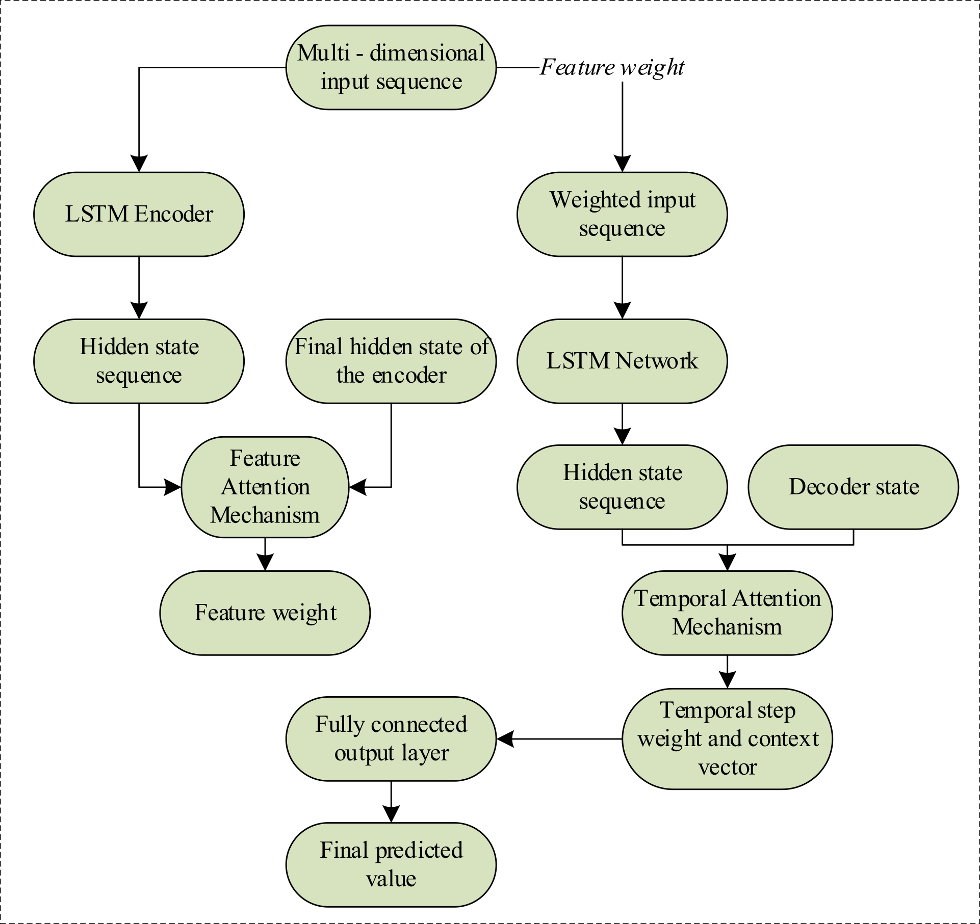
Fig. 1. Detailed architecture of the DA-LSTM model.

Figure 1 shows the detailed architecture of a DALSTM model for PV power prediction. The realisation of this model is mainly divided into three steps: (1) input sequence processing: input multi-dimensional input sequence into multi-layer LSTM network, which extracts preliminary time features and outputs the hidden state of each time step. (2) DA extraction: feature attention generates dynamic feature vectors, while temporal attention generates context vectors containing key historical information. This mechanism enables the model to focus on important input features and related time steps simultaneously. (3) Predictive output: the context vector is transformed through the full connection layer to generate the final power output prediction result.

3.1.2 LSTM module

As the core time processing unit of the model, LSTM can capture the complex correlations in PV power fluctuations. Compared with a standard recurrent neural network (RNN), LSTM adopts gating mechanism, which effectively alleviates the problem of gradient disappearance, making it especially suitable for renewable energy time series with great fluctuation and high uncertainty [15–17]. Figure 2 shows the overall operation framework of LSTM.

In Fig. 2, the operations of the LSTM unit at each time step t involves three gates and the update of the internal cell state. The fundamental computation process is as follows:

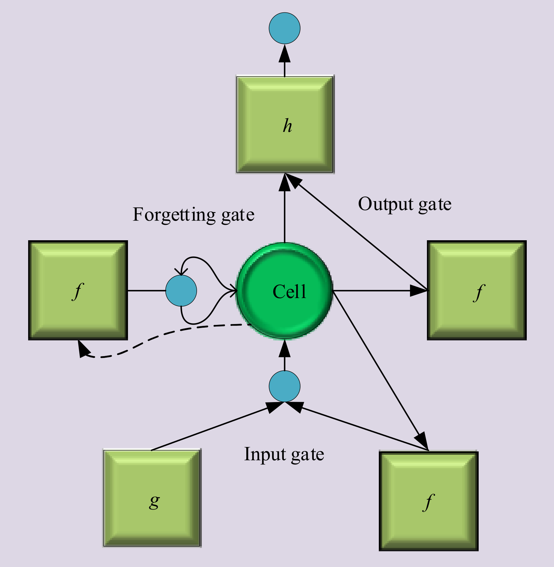
Fig. 2. Schematic diagram of an LSTM unit.

1) Forget gate.

Used to determine which information from the previous cell state should be discarded:

2) Input gate.

Used to control the new information and store it in the cell state:

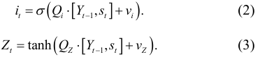
3) Cell state update:

4) Output gate determines which part of the current cell state is output as the hidden state:

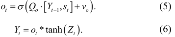
In (1)–(6), s_t represents the input vector at time t (including meteorological data and historical power data), Y_t-1 is the hidden state at time t−1, and Z_t-1 denotes the cell state at time t-1, Q and v correspond to the trainable weight matrices and bias vectors for the respective gates, σ is the sigmoid activation function, producing values between 0 and 1, which simulate the opening and closing of the gates, while tanh adjusts the information flow through non-linear transformation. In this study, multiple LSTM units are stacked to form the encoder, enabling the learning of highdimensional non-linear mappings from the input sequence to the hidden representations. These representations provide temporally rich feature embeddings for the subsequent DA mechanism.

In summary, the LSTM module primarily serves as a time-series feature encoder. Its gating structure provides dynamic memory and forgetting, enabling the model to effectively capture changes in PV power output over time. This robust representation of time-series dependencies underpins the handling of non-stationarity and randomness in renewable energy generation. Furthermore, stacking LSTM layers ensures that the temporal dynamics of the input sequence are fully captured, yielding a dense, information-rich hidden state sequence. This sequence provides a strong foundation for the subsequent highquality feature extraction performed by the DA mechanism.

3.1.3 Integration of DA mechanism

To capture the varying importance of features and historical time steps in PV power sequences, a DA mechanism was integrated into the LSTM model [18]. This mechanism operates on both feature and temporal levels, dynamically adjusting the model focus across the input dimensions [19, 20]. The feature-attention component highlights the most relevant meteorological and operational variables for the current forecasting task by computing attention scores for each feature using a learnable weight matrix [21].

Before computation, the previous time step in the LSTM encoder was set as Y_τ, and an initial input feature matrix was given as R = [r₁, r₂, ..., r_N]. x_i represents the i-th feature variable. The feature attention weight α_i is expressed as:

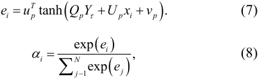
where Q_p, U_p, and u_p are the trainable parameter matrices, and v_p is the bias term. The weighted feature sequence is then constructed as R̃ = [α₁r₁, α₂r₂, ..., α_Nr_N], allowing the model to adaptively emphasise key driving factors such as irradiance under sunny conditions.

A temporal attention mechanism was applied to the hidden state sequence Y′ = [Y′₁, Y′₂, ..., Y′_T], which was obtained after the LSTM processed the weighted feature sequence R̃. It evaluates the relative importance of each historical time step hidden state with respect to the current prediction moment [22, 23]. For the current decoder state s_t, the attention score w_t,i between l_t and the i-th encoder hidden state Y′_i, as well as the corresponding attention weight β_t,i, are computed as follows:

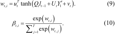
In (9) and (10), Q_t, U_t, and u_t are the trainable parameters, while v_t denotes the bias term [24]. The final context vector is generated as c_t = ∑_j=1^T β_t,iY′_i which integrates information from all time steps most relevant to the current prediction. The purpose of this DA mechanism is to enable the model to identify critical weather features, thereby enhancing the accuracy and stability of PV power output predictions under random fluctuations and sudden weather changes [25, 26].

DA mechanism endows the model with dynamic and adaptive information weighting, enabling high-quality feature extraction. In practical scenarios, the influence of different meteorological variables on PV output varies. For example, in sunny conditions, irradiance plays a leading role. The feature attention and temporal attention components in this model quantify this dynamic importance from two orthogonal dimensions: variable attributes and temporal context. This coordination mechanism enhances the model ability to understand and adapt to a complex, changing environment.

3.1.4 Model fusion and output

After extracting the dynamic information, the model transforms the context vector ct encoding the historically important information into the final power prediction. Specifically, the context vector from the temporal attention layer is directly fed into a fully connected layer. This layer applies a linear transformation using its weight matrix and bias term to produce the predicted output. For regression tasks, the output layer typically omits an activation function to preserve a linear range, which is suitable for continuous target variables such as PV power output. The computation is expressed as follows:

In (11), Q_o and v_o represent the weights and bias of the output layer. Respectively, ŷ_t denotes the model-generated power prediction at time t. This formulation integrates the information selected by the dual attention mechanism with the LSTM-based temporal modelling, meeting the accuracy and reliability requirements for high-penetration renewable energy applications.

The model fusion and output stage serves as the decision-making endpoint of the DA-LSTM model. Here, the context vector encoding key feature information is transformed by a fully connected layer, and the highdimensional feature space is mapped to a single power output value. This design avoids introducing additional complexity while retaining the model feature-extraction ability. In the overall architecture, LSTM captures the time dynamics, the DA mechanism identifies and emphasises key information and the full connection layer performs regression to generate the final prediction result. The integration of these components provides a flexible framework for modelling and quantifying the uncertainty of forecasting.

3.1.5 Model training strategy and optimisation

In order to ensure the efficient learning and strong generalisation ability of the DA mechanism, the model is trained by carefully selected strategies and optimisation techniques. The Huber loss function is adopted as the objective function because it combines the advantages of mean square error (MSE) and mean absolute error (MAE), providing a smooth gradient while reducing sensitivity to outliers. Huber loss function is defined as follows:

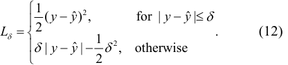
in (12), y and ŷ_t represent the actual and predicted power values, respectively, and δ denotes the threshold hyperparameter.

In order to optimise the model, this study uses Adam optimiser to adaptively control the parameter updating steps to alleviate over-fitting. The learning rate adopts exponential decay strategy, so as to achieve rapid convergence in the initial stage of training and fine adjustment in the later stage. In order to further prevent over-fitting, this study uses Dropout to randomly disable some neurons and apply L₂ regularisation to the fully connected layer. In addition, this study also introduces an early stop mechanism to monitor the performance of the verification set and terminate the training when the performance improvement is stagnant. The main hyperparameter settings are summarised in Table 1.

Table 1.

Model training hyperparameter configuration.

Hyperparameter	Value
Optimiser	AdamW
Training epochs	100
L2 regularisation coefficient	0.001
Batch size	32
Huber loss Threshold (delta)	1.0
Initial learning rate	0.001
Early stopping patience	10
Dropout rate	0.2

3.2 Experimental design for model performance verification

3.2.1 Data source and preprocessing

In order to verify the DA-LSTM model, this study uses a dataset from the CodeChina platform that contains measured data from a grid-connected PV power station in eastern China. The data set spans from January 1st, 2022, to December 31st, 2023, with a time resolution of 15 min, and records the power station temperature, short-term and ultra-short-term PV output power, and solar irradiance (https://gitcode.com/Universal-Tool/cb71e). The prediction task focuses on ultra-short-term PV output power, with the actual PV output power from 15 min ago as the target variable.

In order to ensure data quality, the dataset has been preprocessed systematically. The linear interpolation method is used to keep the continuity of the time series. For occasional negative values caused by measurement error or low reactive power output at night, the historical average of the power station is used to replace them and avoid physically unreasonable values. All features are normalised to the range of [0,1] to eliminate scale differences, accelerate convergence, and enhance model stability. Linear interpolation preserves the smooth temporal trends of PV output and meteorological variables and effectively fills data gaps without distorting the model. Although replacing negative values slightly smooths the extremely low fluctuations, it improves overall data quality and model training performance.

The processed dataset is split into a training set, a verification set, and a test set. Table 2 summarises the division: the training set corresponds to the full year of 2022, the verification set to the first half of 2023, and the test set to the second half of 2023. This time division ensures the independence of the model training period and evaluation period.

Table 2.

Dataset partitioning.

Dataset	Number of samples	Proportion	Purpose description
Training set	5852	70%	Used for model parameter training
Validation set	836	10%	Used for hyperparameter tuning and early stopping
Test set	1672	20%	Used for final model performance evaluation

3.2.2 Experimental environment

All tests are carried out on a unified software and hardware platform. Table 3 provides a detailed overview of the hardware and software configuration.

Table 3.

Experimental configuration.

Category	Item	Configuration / Version
Hardware	GPU	NVIDIA GeForce RTX 3060 Ti (8 GB)
	Central processing unit	Intel Core i7-12700K
	Memory	32 GB
Software	Operating system	Windows 10
	Deep learning framework	PyTorch 2.4.0 + CUDA 12.1
	Programming language	Python 3.9
	Major libraries	NumPy, Pandas, Scikit-learn

3.2.3 Evaluation metrics and baseline models

In this study, three commonly used evaluation indices are used to evaluate the prediction performance of the DALSTM model: 1) root mean square error (RMSE), which is used to quantify the average deviation between the predicted value and the actual value. It is a common index for evaluating and optimising regression models, and is suitable for meteorological forecasting and economic analysis. 2) MAE is defined as the average of absolute errors between the predicted value and the actual value. It reflects the average error size and is not sensitive to abnormal values. 3) The determination coefficient (R²) is used to evaluate the degree to which the regression model can explain the variance of the data. The closer the r value is to 1, the better the fitting degree of the model is.

In addition, several typical baseline models were chosen for comparison with the proposed model to assess its effectiveness and reliability. The baseline models include: Persistence Model (PM), Seasonal Autoregressive Integrated Moving Average (SARIMA), Standard LSTM,

TCN-MHA, Attention-Based Bidirectional LSTM (AttBiLSTM). The informer model, an advanced transformerbased time-series forecasting architecture, achieves efficient long-sequence prediction through a ProbSparse self-attention mechanism and a generative decoder, demonstrating strong performance across multiple timeseries benchmark tasks. All models mentioned above used the official hyperparameter settings, with input sequence lengths matched to those of DA-LSTM, and were trained using the same training strategy and early stopping criteria.

4. Experimental results and analysis

4.1 Comparison of prediction accuracy

This section compares the DA-LSTM model with benchmark models through experiments to verify its effectiveness in forecasting. All baseline models were constructed and trained using the same dataset, input features, and experimental environment, and they employed the same early-stopping strategy as the DALSTM model. The specific configurations of each model were as follows:

• Persistence model (PM): Served as a theoretical baseline and required no training.

• SARIMA: Optimal model orders were determined via grid search.

• Standard LSTM and DA-LSTM: Shared the same encoder architecture, with identical numbers of layers and hidden units; however, the standard LSTM did not include any attention modules.

• TCN-MHA: Followed its standard architecture, employing causal convolutional layers with dilation rates of [1, 2, 4, 8], followed by a four-head attention layer.

• Attention-based BiLSTM (Att-BiLSTM): Utilized a bidirectional LSTM layer and applied a single-head attention mechanism on the hidden state of the final time step.

The comparative results are presented in Figs. 3 and 4. In Figs. 3 and 4, compared with the baseline models, the DA-LSTM model achieves superior performance with an RMSE of 795.36 kW, MAE of 580.15 kW, and R² of 0.9658. Compared with the standard LSTM, the DA-LSTM reduces RMSE by 16.35%, MAE by 18.33%, and improves R² by 2.06%. Relative to the TCN-MHA model, the DA‑LSTM reduces RMSE by 9.68%, MAE by 10.79%, and increases R² by 1.19%. When compared with Att‑BiLSTM,

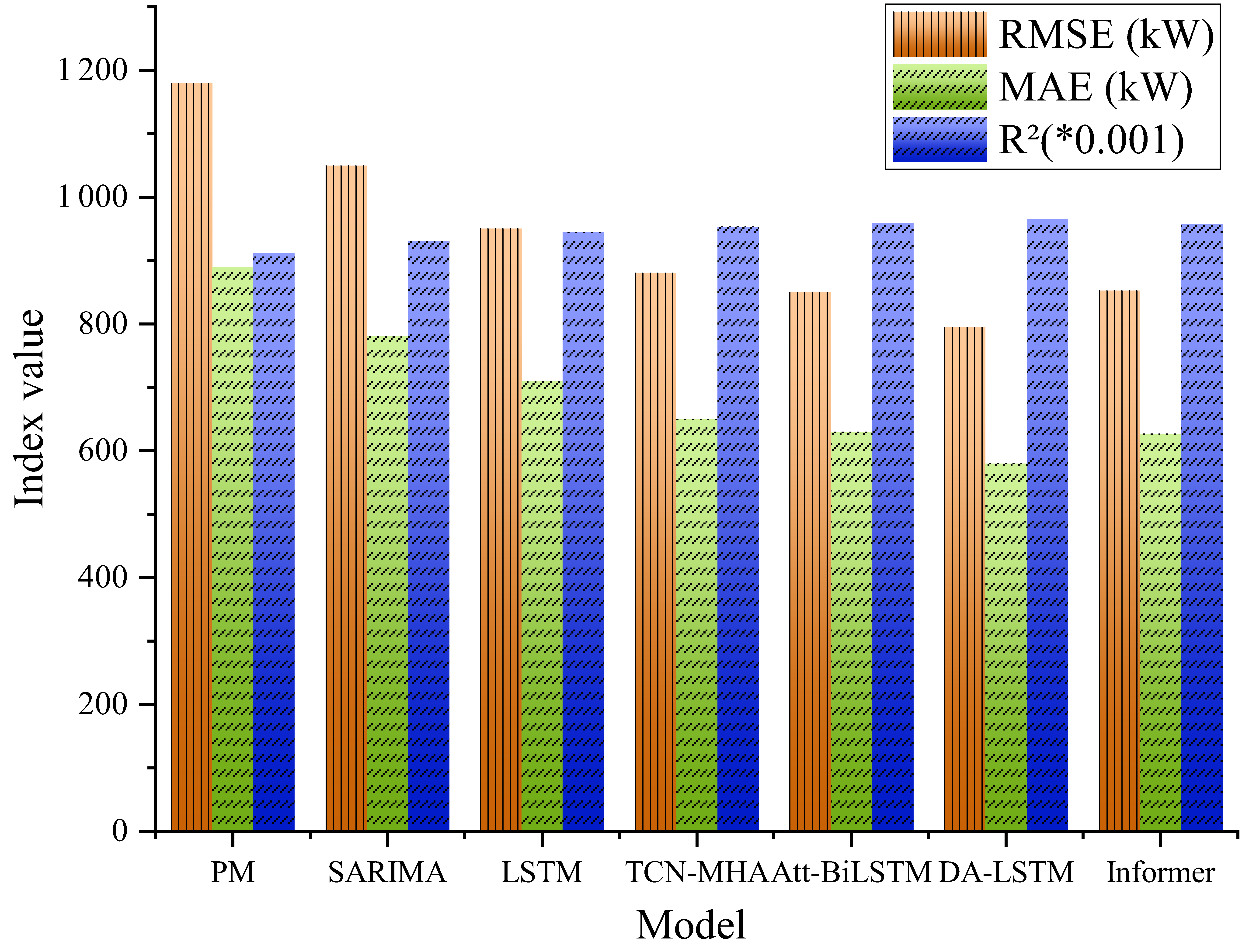
Fig. 3. Comparison of prediction accuracy across models (Test set).

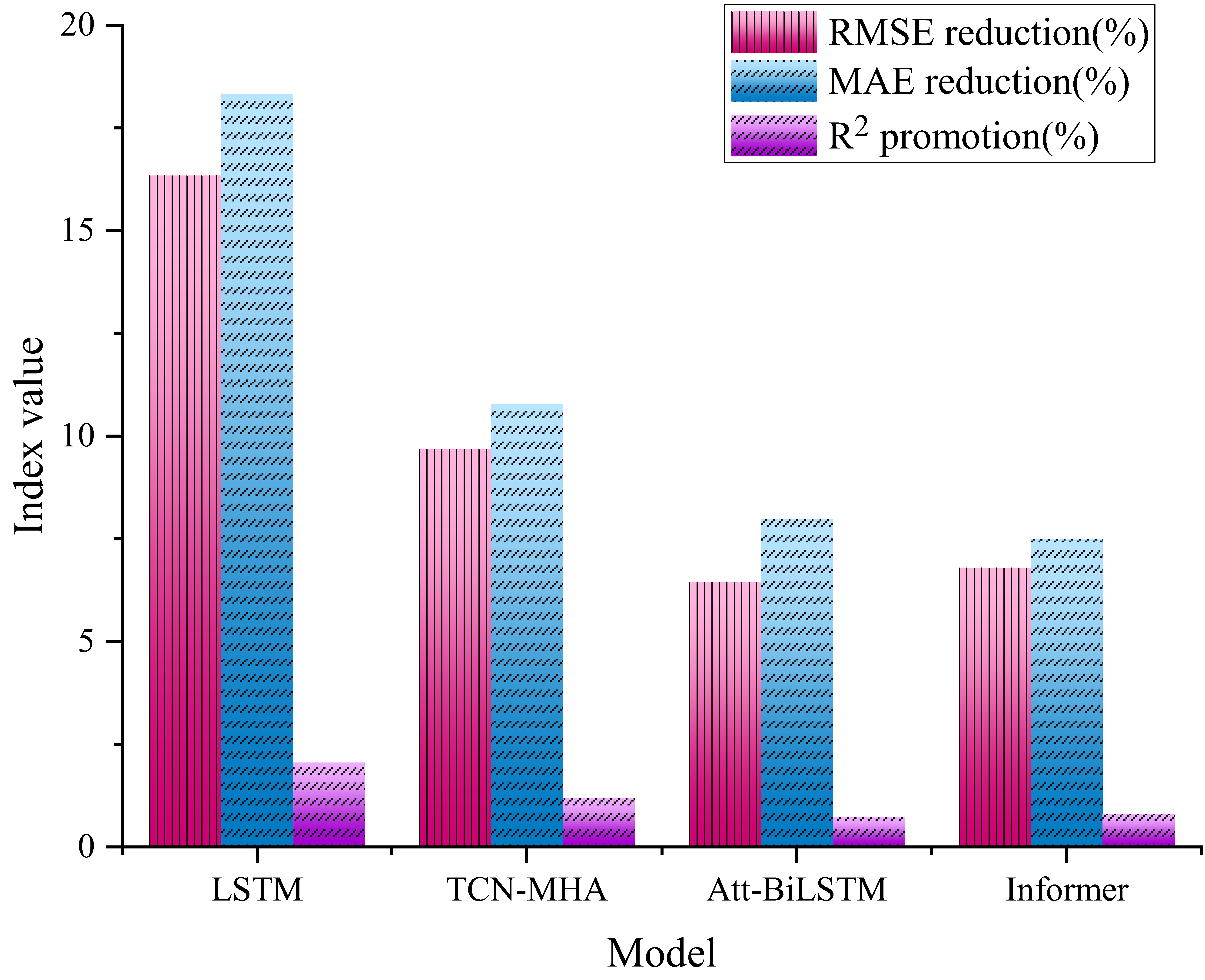
Fig. 4. Relative performance improvements of key models.

DA‑LSTM reduces RMSE by 6.45%, MAE by 7.98%, and increases R² by 0.73%. These results validate that the DALSTM model achieves higher predictive accuracy.

4.2 Effectiveness analysis of the attention mechanism

In this experiment, the two types of attention mechanisms in the model were sequentially removed, and the resulting changes in model performance were observed. In the w/o FAM model, the feature attention module was removed, while in the w/o TAM model, the temporal attention module was removed; all other components remained identical to the full DA-LSTM architecture. All trainable models were trained end-to-end using the same Huber loss function and the AdamW optimiser. Figure 5 presents the model performance before and after removing the two attention mechanisms.

Figure 5 shows that the complete DA-LSTM model has the best performance. After FAM was removed, the performance of the model decreased and RMSE and MAE increased by 4.8% and 5.1%, respectively, indicating that it is very important to identify the weather and business characteristics to improve the forecast accuracy. Similarly, removing TAM also leads to an increase in RMSE and MAE. When both attention mechanisms are removed, the performance degradation is more significant. The analysis shows that FAM and TAM both play an important role in the model.

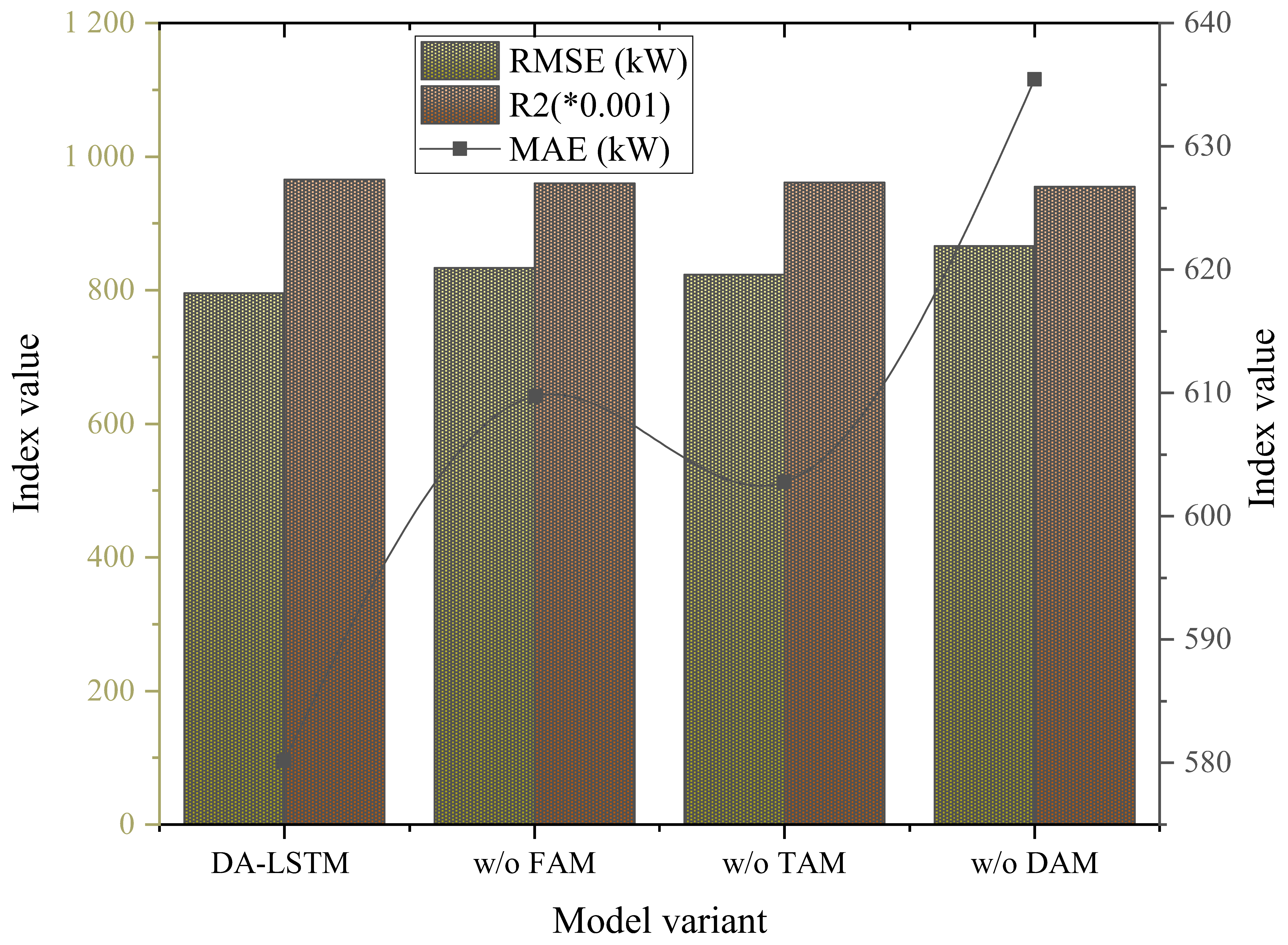
Fig. 5. Relative performance improvements of key models.

In order to further evaluate the performance of the model under complex meteorological conditions, this study compares the complete DA-LSTM model with the standard LSTM model in different weather scenarios, and the results are shown in Fig. 6.

Figure 6 shows that there is little difference in performance between the two models under stable and sunny conditions, and that the DA-LSTM model has a 3.1% lower RMSE than LSTM. However, the RMSE of DA-LSTM decreased by 11.5% and 14.2%, respectively, under cloudy and sunny conditions, and during sudden weather changes. These results show that the dual attention mechanism can effectively deal with complex non-linear events.

After analysing the improvement of prediction accuracy brought by the attention mechanism, this study further investigated the weight distribution of characteristic attention and temporal attention under different weather conditions to explore the physical basis of model decisionmaking. Figure 7 shows the attention weights assigned by the model to input features (irradiance, temperature, humidity, and historical power) in typical sunny, cloudy, and rapidly changing weather scenarios.

As shown in Fig. 7, the irradiance is the highest (0.52) in sunny days, indicating that it is the main driving factor. Under cloudy conditions, the weight of irradiance decreased slightly (0.43), while the weight of temperature and historical power increased, indicating that the model depends on the combination of many factors. In the case of rapid weather changes, the weight of irradiance further drops to 0.31, while the weight of historical power rises to 0.29, indicating that the model tends to capture abrupt changes by emphasising historical trends.

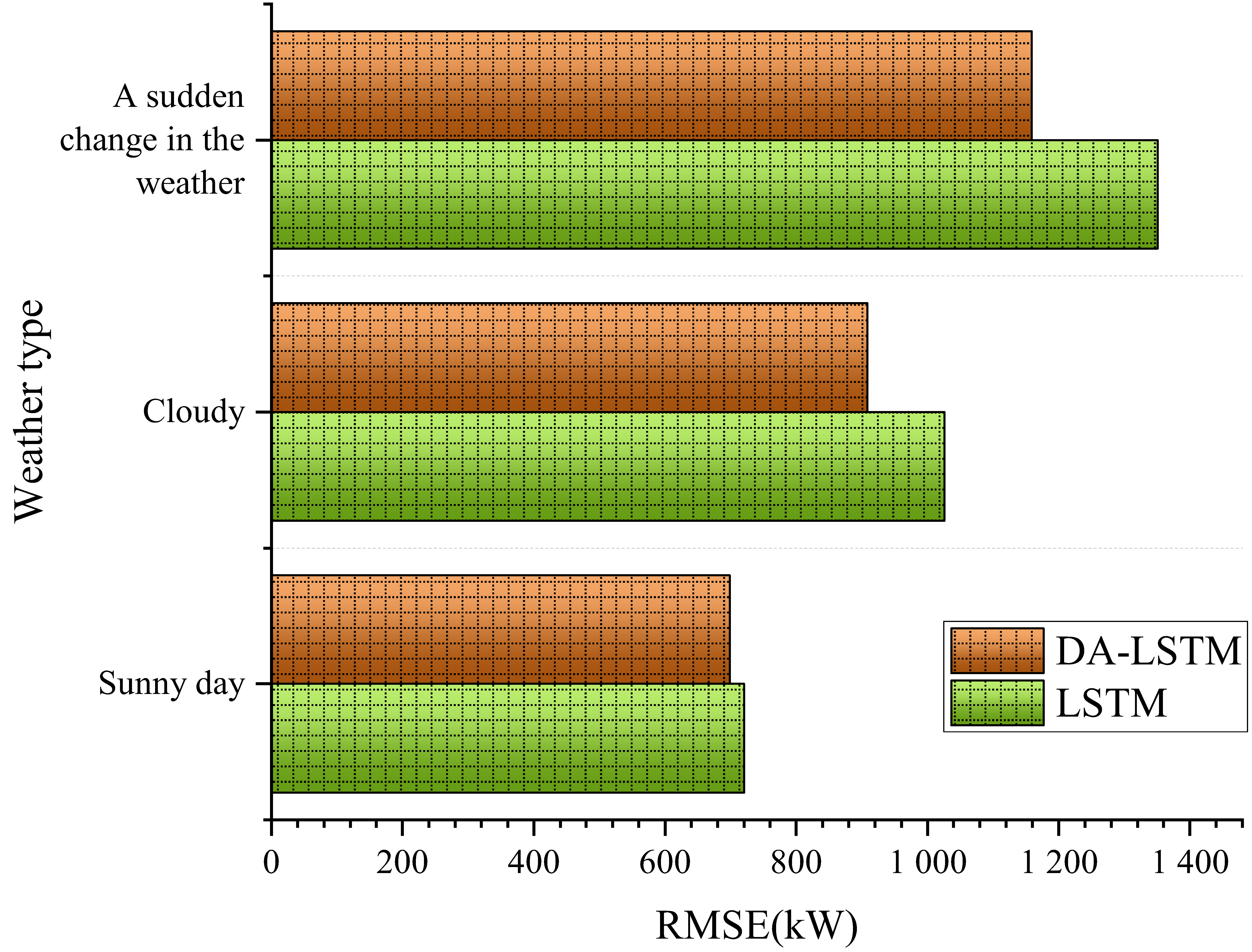
Fig. 6. Model prediction effect comparison under different weather conditions (RMSE: kW).

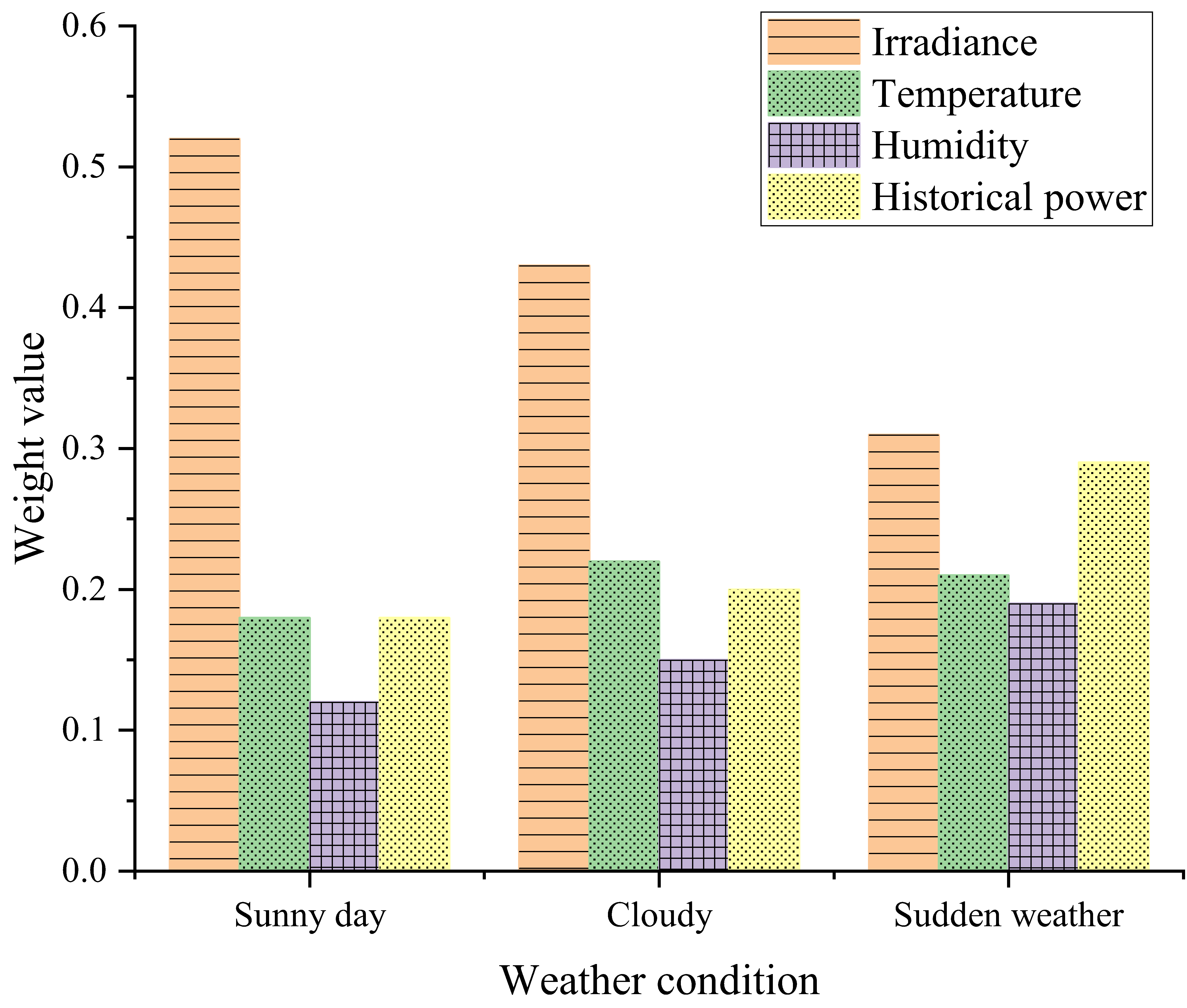
Fig. 7. Attention weights of key features under different weather conditions.

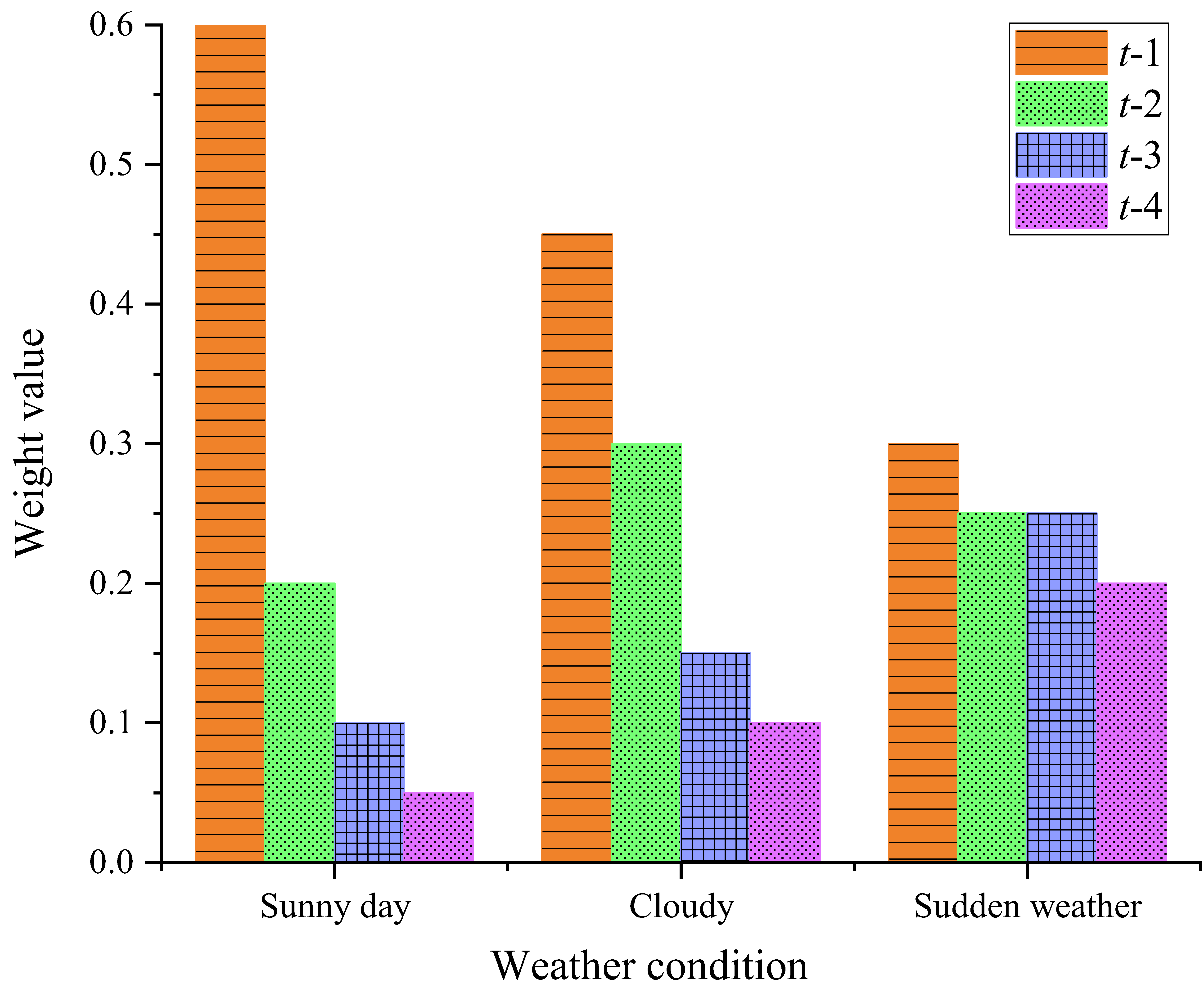
Fig. 8. Temporal attention weight distributions under different weather conditions.

In order to study the behaviour of the time attention mechanism under different meteorological conditions, this study selected representative samples of sunny days, cloudy days, and rapid weather changes from the test set. Then, this study calculates the average attention weight assigned to the last four historical time steps (t −1 to t −4) at the time of prediction. The result is shown in Fig. 8.

As shown in Fig. 8, under clear conditions, the model mainly focuses on the nearest time step (t −1 weight = 0.65), which is in line with physical intuition, that is, under stable weather conditions, the PV output will change gradually, and the latest observation data have the most reference value. On cloudy days, due to irradiance fluctuations caused by cloud cover, the weights for t −1 and t −2 are similar, indicating that more historical information is needed to capture the changing trend. In the case of rapid weather changes, the weight of concern is more evenly distributed among historical steps, and the differences between them are smaller. This shows that the model will automatically increase its reliance on historical information to cope with the violent fluctuations in output. These observations confirm that the time attention mechanism dynamically adjusts its attention to the historical window based on environmental conditions, thus improving the stability and adaptability of the forecast.

4.3 Adaptability verification under high-penetration scenarios

This study focuses on the prediction performance of a DA‑LSTM model under the condition of high renewable energy permeability, as shown in Table 4. In this study, a “high-permeability scenario” was constructed based on the historical output data of the experimental PV power station. The power station output value is scaled to simulate its contribution under different regional load shares, thus creating simulation datasets with permeability levels of 20% and 40%, respectively.

Table 4.

Model performance comparison under different renewable energy penetration levels.

Penetration scenario	Model	RMSE (kW)	MAE (kW)
20% Penetration	LSTM	950.75	710.48
	DA-LSTM	795.36	580.15
40% Penetration	LSTM	1123.79	845.62
	DA-LSTM	985.25	746.91

Table 4 shows that when the permeability is 20%, the RMSE and MAE of the DA-LSTM model are lower than those of the standard LSTM model, indicating that the DA‑LSTM can achieve a better prediction performance even at low permeability. With permeability increased to 40%, the fluctuation of system net load is more significant, leading to the increase of prediction errors of all models.

However, the DA-LSTM model remains superior to other models, and the error fluctuation is better controlled, which shows its ability to effectively handle fluctuations in highpermeability scenarios.

In the above experiments, 20% and 40% highpermeability scenarios were initially simulated by scaling the historical output data of a single PV power station. The advantage of this method is that it can effectively reflect the key feature of high permeability, that is, PV power generation accounts for a larger proportion of the net load. By scaling the output of a single power station while keeping other variables unchanged, the amplified net load fluctuation can be simulated, and the forecasting performance of the model can be observed as the fluctuation of PV power generation increases. However, this method has limitations. It simplifies the spatiotemporal smoothing effect of multiple PV power stations in the actual power grid and fails to fully capture the complex power flow distribution and dynamic interactions, such as reductions in system inertia and increase of frequency adjustment pressure in high-permeability networks.

In order to overcome these limitations, this study further incorporates operational data of regional power grids and constructs two system-level verification scenarios with different permeability characteristics. Scenario A represents a regional power grid with a PV penetration rate of about 20%, while scenario B represents a power grid with a PV penetration rate close to 40%. The data includes the aggregate output of several distributed PV power plants and the corresponding net load in each period. Table 5 summarises the model prediction performance in these scenarios.

Table 5.

Model prediction performance under different high-penetration system-level scenarios.

Penetration scenario	Model	RMSE (MW)	MAE (MW)
20% Penetration	LSTM	9.51	7.12
	DA-LSTM	8.23	6.05
40% Penetration	LSTM	18.45	14.38
	DA-LSTM	15.92	12.17

As shown in Table 5, the DA-LSTM model is superior to the standard LSTM model in both scenarios, yielding lower RMSE and MAE values. This shows that the DA‑LSTM model can effectively capture the violent fluctuation of net load under the high-permeability condition, even if there are spatio-temporal smoothing effects of multiple PV power plants, which proves its effectiveness and stability in a complex system environment.

Since the model is intended for PV power prediction, it is crucial to evaluate its predictive stability in different permeability scenarios. Therefore, this study conducted a statistical analysis of the forecasting performance of different models across varying penetration rates. The results are presented in Fig. 9.

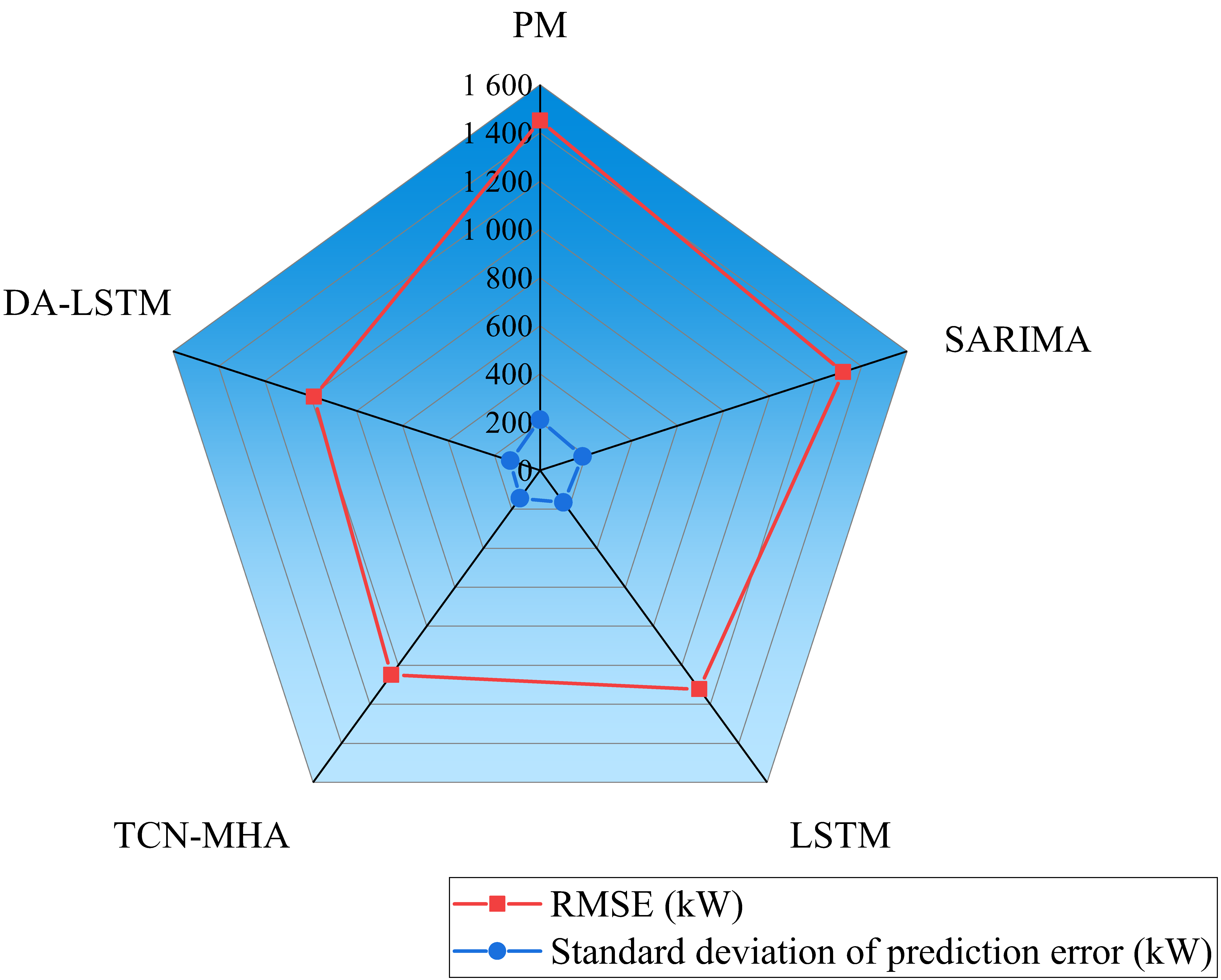
Fig. 9. Comparison of prediction error variability under highpenetration scenario (40% penetration).

As shown in Fig. 9, compared with the baseline models, the DA-LSTM model achieves a prediction error of 128.7 kW, indicating higher accuracy and greater reliability. Further analysis reveals that the DA-LSTM model is better able to cope with strong fluctuations and uncertain conditions in high-penetration power systems.

4.4 Analysis of computational efficiency

This study compared the operational costs of the DALSTM model with benchmark models, focusing on the number of model parameters, training time per epoch, and prediction time per batch, as illustrated in Fig. 10.

Figure 10 shows that incorporating the DA mechanism increased the number of parameters in the DA-LSTM model to 1.82 M, which is higher than that of the standard LSTM (1.15 M) and TCN-MHA (1.45 M), and the training time per epoch reached 125 s. However, the prediction time per batch was only 15.3 ms. Although slightly higher, this value meets the real-time requirements of short-term forecasting tasks. These results show that although the prediction accuracy of the DA-LSTM model is higher, its operating cost also increases.

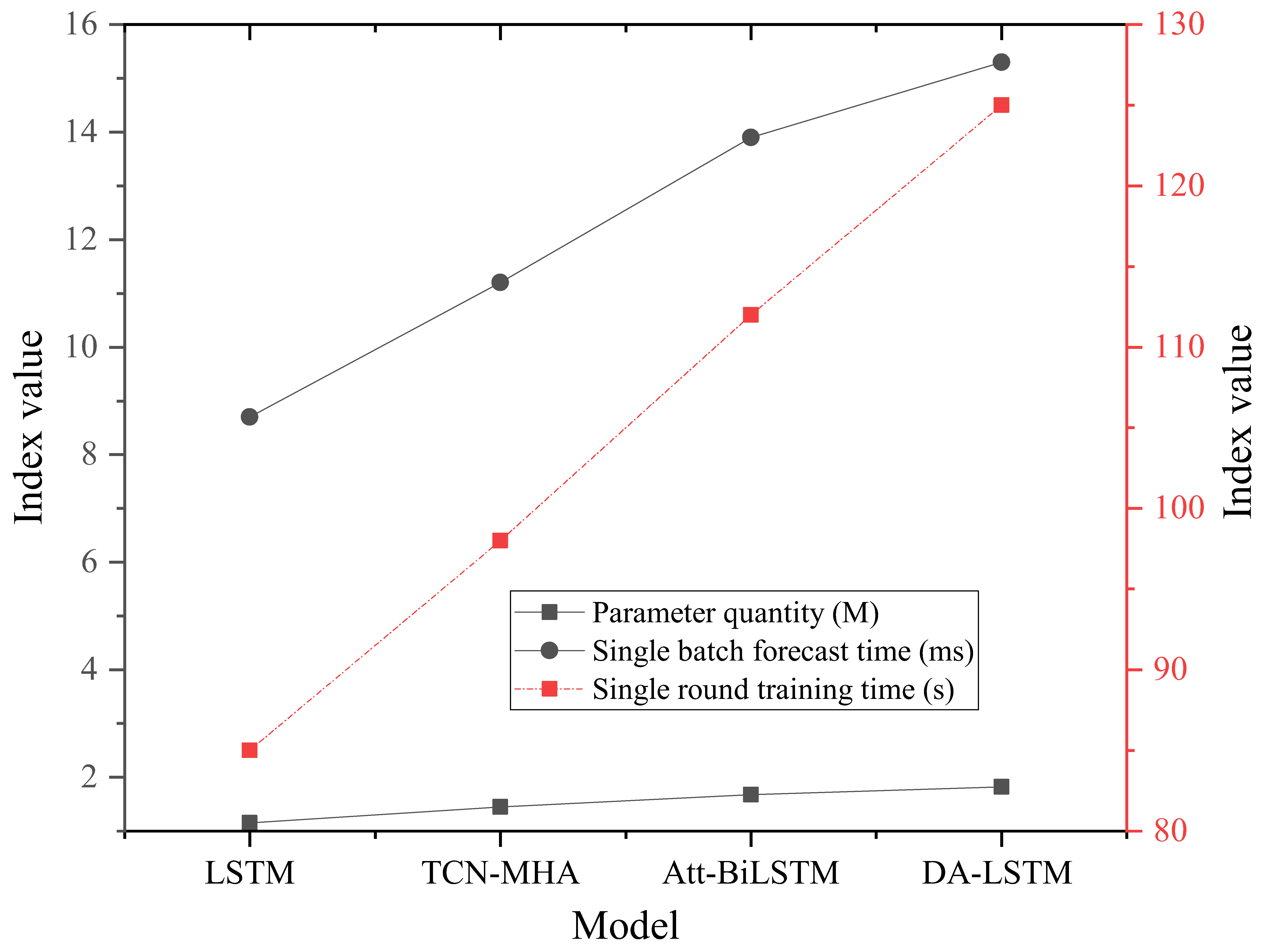
Fig. 10. Comparison of model computational efficiency.

4.5 Data quality robustness analysis

To evaluate the model performance when data quality degrades in the actual engineering setting, this study conducted robustness experiments involving data loss and noise interference. Firstly, the random missing rates of 5% and 10% are introduced into the original test set, and three interpolation strategies are compared: linear interpolation, mean filling, and forward filling. Secondly, different levels of Gaussian noise (SNR is 20 dB and 15 dB, respectively) are added to simulate the measurement error. Finally, this study compares outlier-processing strategies, including median filtering and 3 σ truncation. The results are summarised in Tables 6–8.

Table 6.

Model prediction performance under different missing rates (RMSE in kW).

Missing rate	LSTM	TCN- MHA	Att- BiLSTM	Informer	DA-LSTM
0%	900.42	830.17	850.83	853.27	795.36
5%	978.65	908.33	929.71	933.54	848.92
10%	1067.31	998.65	1021.44	1024.18	908.75

Table 7.

Model prediction performance under different noise levels (RMSE in kW).

Noise level	LSTM	TCN- MHA	Att- BiLSTM	Informer	DA-LSTM
No noise	900.42	830.17	850.83	853.27	795.36
SNR = 2 dB	950.23	880.45	901.12	904.56	830.21
SNR = 15 dB	998.72	928.34	950.67	953.89	862.44

Table 8.

DA-LSTM performance under different outlier handling strategies.

Handling strategy	RMSE (kW)	MAE (kW)
None	862.44	642.18
3σ truncation	848.91	631.45
Median filtering	823.57	610.32

As Tables 6–8 suggest, as the missing rate increases, the prediction errors of all models increase. However, the error increase of DA-LSTM is the smallest. In the noise experiment, when the SNR drops to 15 dB, the RMSE of DA-LSTM is 862.44 kW, which is still lower than that of other models at the same noise level (e.g., LSTMs RMSE is 998.72 kW). In addition, the comparison of outlier processing strategies shows that median filtering can further reduce RMSE compared with 3 σ truncation. These results show that DA-LSTM can still maintain relatively stable prediction performance under different data quality because of its DA mechanism that emphasises key features. This proves its robustness and reliability in a real deployment scenario.

4.6 Discussion

The above analysis shows that combining the DA mechanism with the LSTM model can significantly improve the prediction performance. Compared with the traditional LSTM model or a model that uses only a single attention mechanism, the DA mechanism can extract key information from input data more effectively. The feature attention module can automatically identify and emphasise the most influential factors under current meteorological conditions. At the same time, the time attention module focuses on the historical time step that is most relevant to the forecast time limit, so as to ensure that a stable forecast can be made even in the case of rapid weather fluctuation or sudden changes. These mechanisms jointly enhance the modelling ability of the model for non-linear time dependence and improve the adaptability of the model to a complex and changeable operating environment.

5. Conclusions

With the increasing penetration rate of renewable energy in the power grid, accurate PV power generation prediction has become increasingly important. In order to meet this challenge, this study proposes a DA-LSTM model with a DA mechanism, which pays attention to both feature and time series. By combining feature attention and time attention, the model can dynamically identify key meteorological factors and the most relevant historical time step. The experimental results show that the RMSE of the model is 795.36 kW, the MAE is 580.15 kW, and the correlation coefficient (r) is 0.9658, indicating higher robustness compared with the standard LSTM model.

Although the DA-LSTM model has strong prediction performance, it still has some limitations. Firstly, the DA mechanism increases the number of parameters, which leads to the extension of training time and the increase of calculation. Secondly, the model is only verified on the data of a single PV power station, and its generalisation ability to wind power or other renewable energy scenarios has not been verified. Thirdly, the model is sensitive to the quality of input data, and the lack of data or noise data will lead to a decline of model performance. Future research will focus on the design of lightweight models using pruning or quantisation techniques. In addition, the model prediction ability should be tested in several renewable energy systems, and a wider range of meteorological and operational variables should be included. These steps aim to improve the model practicability, adaptability, and robustness in a changeable environment.

Funding

This work was supported by the Doctoral Research Startup Fund of Nantong Institute of Technology, China (Grant No. 2025XKB19).

References

[1] Swadi, M. et al. Investigating and predicting the role of PV, wind, and hydrogen energies in sustainable global energy evolution. Glob. Energy Interconnect. 7, 429–445 (2024). https://doi.org/10.1016/j.gloei.2024.08.009

[2] Iheanetu, K. J. Solar PV power forecasting: A review. Sustainability 14, 17005 (2022). https://doi.org/10.3390/su142417005

[3] Sun, K. et al. Output power prediction of stratospheric airship solar array based on surrogate model under global wind field. Chin. J. Aeronautics 38, 103244 (2025). https://doi.org/10.1016/j.cja.2024.09.020

[4] Karaman, Ö. A. et al. Prediction of wind power with machine learning models. Appl. Sci. 13, 11455 (2023). https://doi.org/10.3390/app132011455

[5] Tsai, W.-C., Tu, C.-S., Hong, C.-M. & Lin, W.-M. A review of state-of-the-art and short-term forecasting models for solar PV power generation. Energies 16, 5436 (2023). https://doi.org/10.3390/en16145436

[6] Hajjaj, C. et al. Comparing PV power prediction: Ground-based measurements vs. satellite data using an ANN model. IEEE J. Photovolt. 13, 998–1006 (2023). https://doi.org/10.1109/JPHOTOV.2023.3306827

[7] Wang, Y. et al. The wind and PV power forecasting method based on digital twins. Appl. Sci. 13, 8374 (2023). https://doi.org/10.3390/app13148374

[8] Wu, Z. et al. Prediction of PV power by the informer model based on convolutional neural network. Sustainability 14, 13022 (2022). https://doi.org/10.3390/su142013022

[9] Ge, W. & Wang, X. PSO–LSTM–Markov coupled PV power prediction based on sunny, cloudy and rainy weather. J. Electr. Eng. Technol. 20, 935–945 (2025). https://doi.org/10.1007/s42835-024-02051-y

[10] Luo, Y., Wang, Y., Liu, C. & Fan, L. Two‐stage robust optimal scheduling of wind power‐PV‐thermal power‐pumped storage combined system. IET Renew. Power Gener. 16, 2881–2891 (2022). https://doi.org/10.1049/rpg2.12544

[11] Mahjoub, S., Chrifi-Alaoui, L., Drid, S. & Derbel, N. Control and implementation of an energy management strategy for a PV–wind– battery microgrid based on an intelligent prediction algorithm of energy production. Energies 16, 1883 (2023). https://doi.org/10.3390/en16041883

[12] El Bourakadi, D., Ramadan, H,, Yahyaouy, A. & Boumhidi, J. A novel solar power prediction model based on stacked BiLSTM deep learning and improved extreme learning machine. Int. J. Inf. Technol. 15, 587–594 (2022). https://doi.org/10.1007/s41870-022-01118-1

[13] Alkesaiberi, A., Harrou, F. & Sun, Y. Efficient wind power prediction using machine learning methods: A comparative study. Energies 15, 2327 (2022). https://doi.org/10.3390/en15072327

[14] Malik, P., Gehlot, A., Singh, R., Gupta, L. R. & Thakur, A. K. A review on ANN based model for solar radiation and wind speed prediction with real-time data. Arch. Comput. Methods Eng. 29, 3183–3201 (2022). https://doi.org/10.1007/s11831-021-09687-3

[15] Wang, J. et al. Two-stage energy management strategies of sustainable wind-PV-hydrogen-storage microgrid based on receding horizon optimization. Energies 15, 2861 (2022). https://doi.org/10.3390/en15082861

[16] Khan, K. I. & Nasir, A. Application of artificial intelligence in solar and wind energy resources: A strategy to deal with environmental pollution. Environ. Sci. Pollut. Res. 30, 64845– 64859 (2023). https://doi.org/10.1007/s11356-023-27038-6

[17] Xiang, X., Li, X., Zhang, Y. & Hu, J. A short-term forecasting method for PV power generation based on the TCN-ECANet-GRU hybrid model. Sci. Rep. 14, 6744 (2024). https://doi.org/10.1038/s41598-024-56751-6

[18] Patel, A. et al. A practical approach for predicting power in a small-scale off-grid PV system using machine learning algorithms. Int. J. Photoenergy 2022, 9194537 (2022). https://doi.org/10.1155/2022/9194537

[19] Huang, Z., Huang, J. & Min, J. SSA-LSTM: Short-term PV power prediction based on feature matching. Energies 15, 7806 (2022). https://doi.org/10.3390/en15207806

[20] Cebekhulu, E., Onumanyi, A. J. & Isaac, S. J. Performance analysis of machine learning algorithms for energy demand–supply prediction in smart grids. Sustainability 14, 2546 (2022). https://doi.org/10.3390/su14052546

[21] Sun, Y. et al. Nonparametric probabilistic prediction of regional PV outputs based on granule-based clustering and direct optimization programming. J. Mod. Power Syst. Clean Energy 11, 1450–1461 (2023). https://doi.org/10.35833/MPCE.2022.000577

[22] Zhang, X. et al. Digital twin empowered PV power prediction. J. Mod. Power Syst. Clean Energy 12, 1472–1483 (2023). https://doi.org/10.35833/MPCE.2023.000351

[23] Gao, H. et al. Short-term prediction of PV power based on combined modal decomposition and NARX-LSTM-LightGBM. Sustainability 15, 8266 (2023). https://doi.org/10.3390/su15108266

[24] Abualigah, L. et al. Wind, solar, and PV renewable energy systems with and without energy storage optimization: A survey of advanced machine learning and deep learning techniques. Energies 15, 578 (2022). https://doi.org/10.3390/en15020578

[25] Yuan, D.-D., Li, M., Li, H.-Y., Lin, C.-J. & Ji, B.-X.Wind power prediction method: Support vector regression optimized by improved jellyfish search algorithm. Energies 15, 6404 (2022). https://doi.org/10.3390/en15176404

[26] Kassem, Y. & Othman, A. A. Selection of most relevant input parameters for predicting PV output power using machine learning and quadratic models. Model. Earth Syst. Environ. 8, 4661–4686 (2022). https://doi.org/10.1007/s40808-022-01413-7