Analysis of nonlinear response of anti-parity-time symmetric structure

1. Institute of Microelectronics and Optoelectronics, Warsaw University of Technology, ul. Koszykowa 75, 00-665 Warsaw, Poland
2. National Institute of Telecommunications, ul. Szachowa 1, 04-894 Warsaw, Poland

Abstract

This paper presents a theoretical analysis of a gain and loss saturation effect in planar multilayer anti-parity-time (APT) symmetric structures for the first time. This analysis makes it possible to examine the behaviour of nonlinear APT structures when excited by incident light of known intensity and compare their properties with corresponding paritytime (PT) symmetric structures. Two types of APT structures are studied: one with both layers of the primitive cell being gain layers and the other with both layers being loss layers. The refractive indices of the individual layers satisfy the condition n(z) = ‒n*(‒z). Nonlinear analysis is performed using a modified transfer matrix method, which allows for the determination of output intensity characteristics as a function of input intensity for different levels of gain or loss saturation intensities. These characteristics demonstrate a bistable behaviour and a strong nonreciprocal response of the investigated APT structures. The results obtained for both types of APT structures are compared with corresponding PT structures, showing that APT structures reveal identical linear and nonlinear responses as corresponding PT structures.

Introduction

Structures exhibiting anti-parity-time (APT) symmetry have been studied since the second decade of the 21st century [1] and their predecessors, i.e., parity-time (PT) symmetric structures since the end of the 20th century [2]. The principle of creating PT structures in photonics is related to the refractive index [3] of two layers creating a periodic lattice. These layers are characterized by complex refractive indices n = n_Re + in_Im that satisfy the following condition n(z) = n*(‒z), where the asterisk denotes a complex conjugate. This condition can be rewritten separately for the real and imaginary parts of the refractive index of two layers, i.e., n_Re(z) = n_Re(‒z) (the real parts are equal) and n_Im(z) = ‒n_Im(‒z) (the imaginary parts are the additive inverse of each other). The condition for the imaginary part is implemented by using two optically active materials: amplifying (n_Im < 0) and absorbing (n_Im > 0).

In APT symmetric structures, the complex refractive index is consistent with the relationship of n(z) = ‒n*(‒z), i.e., its real and imaginary parts fulfil the conditions of n_Re(z) = ‒n_Re(‒z) and n_Im(z) = n_Im(‒z) [1], which means that the primitive cell of the APT structure may consist of two gain layers or two loss layers. These structures demonstrate unique properties in the absence of any gain medium, such as: spontaneous phase transition of the S matrix [1], continuous lasing spectrum [1], total flat transmission band [1], unidirectional invisibility [4], and reflection anisotropy for light waves incident from two opposite directions [5].

Designing the APT structure requires the usage of a negative index material (NIM). This can be achieved by using a new class of metamaterials in the optical field [6], such as special photonic crystals like nano-fishnets with voids of various shapes. The optical loss of the APT structure (corresponding to the positive imaginary part of the refractive index) can be regulated by ion doping [7]. The optical gain (the negative imaginary part of the refractive index) can be achieved by using quantum wells [8] or nonlinear two-wave mixing [9].

APT symmetric structures are theoretically investigated in various arrangements such as: dissipatively coupled optical structures, where a flat broadband light transport and dispersion-induced dissipation are observed [10], single-particle sensor based on the APT symmetric indirectly coupled whispering gallery mode (WGM) cavities [11], optical gyroscope using APT symmetry, characterized by greater sensitivity than classic systems [12], APT highsensitivity sensor [13], and single damping linear resonator with APT symmetry [14].

The first works with physical implementations of the APT structures have already appeared. One is an on-chip realization of the APT symmetry structure using a fully passive, nanophotonic platform consisting of three evanescently coupled waveguides [15]. The next one demonstrates the APT symmetry in a spectral dimension induced by a nonlinear Brillouin scattering in a single optical microcavity [16]. The newest one shows an on-chip chiral polarizer by constructing a polarization-coupled APT symmetric system [17].

The analyses of the APT structures published so far [1, 4, 5] presented their transmission properties without considering saturation effects. Therefore, in this work, a nonlinear response of the multilayer APT symmetric structure is investigated, taking into account the gain and loss saturation effects. The proposed simple model shows the output intensity as a function of the input intensity of the plane wave illuminating the studied structure for different levels of gain and loss saturation intensities. This model enables the examination of the finite APT structure composed of any optical material. Moreover, it considers the refractive index of the medium surrounding the structure. This is important in the applications of the analysed structures, where they can be an element of an integrated system or a stand-alone device (e.g., a mirror or a filter) in optical hybrid systems. Furthermore, the investigation is carried out for the APT structures, without loss of generality, working at a wavelength equal to 1.55 um, which is typical for telecommunication systems.

The study of the APT symmetric structure is performed using a modified transfer matrix method [18] which was adapted to take into account for the gain and loss saturation effects and the incident wave intensity [19]. The proposed model allows easy examination of gain and loss saturation levels influence on output intensities.

Firstly, the method of determining the refractive indices of the APT structure is presented. Next, the structure is analysed regardless of gain and loss saturations to obtain its geometrical parameters. This linear analysis identifies optimal points where the reflection and transmission coefficients are at their maximum (their values are much higher than unity). The results of this analysis are compared with the results of the analysis of corresponding PT structures. Further, the study is conducted to analyse different levels of the gain and loss saturation intensity parameters for multilayer APT and corresponding PT structures. The obtained characteristics of the output intensities demonstrate a bistable behaviour. The following section presents a theory describing the APT structure. In section 3, the charts illustrate the longitudinal distribution of the field and the characteristics showing the output intensity as a function of the input intensity for different levels of gain and loss saturation intensities. Section 4 presents the conclusions. Appendices contain a more detailed description of the numerical analysis, as well as the field distribution of the compared APT and corresponding PT structures.

Theory

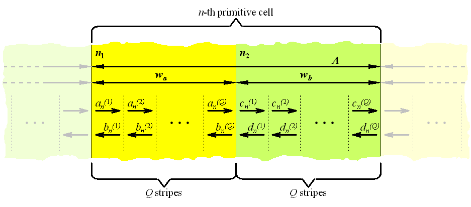
The APT symmetric periodic structure under investigation, shown in Fig. 1, comprises alternating layers characterized by complex refractive indices. One layer has a refractive index of n₁; the other one has n₂. The refractive index of a surrounding medium is n₀. Fig. 1 presents two setups: setup 1 when the wave illuminates the layer with the refractive index n₁ [Fig. 1(a)], setup 2 when the wave illuminates the layer with the refractive index n₂ [Fig. 1(b)].

‌

For the PT structure, refractive indices have to satisfy the following condition n(z) = n*(‒z) which implies the form of these coefficients:

\( \text { PT: } \quad n_1=n_{R e}-i n_{I m}, \quad n_2=n_{R e}+i n_{I m} \) (1)

where n_Re and n_Im are the real and imaginary parts, respectively. Whereas, for the APT structure, refractive indices have to satisfy the APT condition n(z) = ‒n*(‒z). This condition allows for the selection of the refractive indices of the APT structure in relation to the PT structure. In the first case, if the layer with the index n₁ is gain (as in the PT structure), the refractive index of the second APT layer n₂ is chosen according to the above condition. Then, both layers of the APT structure have a negative imaginary part of the refractive index n_Im and will be referred to as APT_gain. In the second case, if the layer with the index n₂ is loss (as in the PT structure), the refractive index of the second APT layer n₁ is selected according to the same condition. Then, both layers of the APT structure have a positive refractive index n_Im and will be referred to as APT_loss. It is worth noting that for both cases, the real parts of the refractive indices have opposite signs, respectively in APT_gain and in APT_loss, as shown below:

\( \begin{array}{ll} \mathrm{APT}_{\text {gain }}: & n_1=n_{R e}-i n_{I m} \Rightarrow n_2=-n_{R e}-i n_{I m} \\ \mathrm{APT}_{\text {loss }}: & n_2=n_{R e}+i n_{I m} \Rightarrow n_1=-n_{R e}+i n_{I m} \end{array} \) (2)

The analysed APT (or PT) structure comprises primitive cells with two layers characterized by equal widths wa = wb. The size of the primitive cell is denoted by Λ = w_a + w_b. The length of the entire structure depends on the number of primitive cells N and their size Λ, i.e., L = NΛ.

The electric field distribution within the first layer E_1n(x) and the second layer E_2n(x) can be written as a sum of two plane waves travelling in the positive and negative direction of the X axis, respectively (see Fig. 1). According to [20], the complex amplitudes of each wave in the n-th cell are the following:

\( \begin{aligned} & E_{1 n}(x)=a_n \cdot e^{\left(i k_0 n_1 x\right)}+b_n \cdot e^{\left(-i k_0 n_1 x\right)} \\ & E_{2 n}(x)=c_n \cdot e^{\left(i k_0 n_2 x\right)}+d_n \cdot e^{\left(-i k_0 n_2 x\right)} \end{aligned} \) (3)

where an and bn are the electric field complex amplitudes of counter running waves in the first layer, cn and dn in the second one, and k0 is the wave number in the free space.

Linear case

In this section, the linear analysis of the APT or PT symmetric structures is presented using the modified transfer matrix method [18, 20], neglecting gain and loss saturation effects. In this work, the plane wave is normally incident on the APT (or PT) symmetric structure only on one side, i.e., on the layer with the refractive index n₁ or n₂. Therefore, depending on which layer the wave is incident upon, its intensity equals I_in (1) = |c0|² for setup 1 [Fig. 1(a)] or I_in (2) = |a0|² for setup 2 [Fig. 1(b)]. Simultaneously, the analysed wave is reflected with an intensity equal to I^r(1) = |d0|² or I^r(2) = |b0|² and the output wave is equal to I_out(1) = |aN+1|² or I_out(2) = |cN+1|², respectively.

The transfer matrices M^(1,lin) and M^(2,lin) are comprised of the junction J and the propagation P matrices (see Fig. 1). For waves illuminating the first or second layer of the APT (or PT) structure, respectively, they are defined for one (N = 1) or more primitive cells (N > 1) as follows:

\( \begin{aligned} & N=1 \Rightarrow\left\{\begin{array}{l} M^{(1, \text { lin })}=J_{01}^{(\text {lin })} P_1^{(\text {lin })} J_{12}^{(\text {lin })} P_2^{(\text {lin })} J_{20}^{(\text {lin })}, \\ M^{(2, \text { lin })}=J_{02}^{(\text {lin })} P_2^{(\text {lin })} J_{21}^{(\text {lin })} P_1^{(\text {lin })} J_{10}^{(\text {lin })}, \end{array}\right. \\ & N>1 \Rightarrow\left\{\begin{array}{l} M^{(1, \text { lin })}=J_{01}^{(\text {lin })}\left(\prod_1^{N-1} P_1^{(\text {lin })} J_{12}^{(\text {lin })} P_2^{(\text {lin })} J_{21}^{(\text {lin })}\right) P_1^{(\text {lin })} J_{12}^{(\text {lin })} P_2^{(\text {lin })} J_{20}^{(\text {lin }),} \\ M^{(2, \text { lin })}=J_{02}^{(\text {lin })}\left(\prod_1^{N-1} P_2^{(\text {lin })} J_{21}^{(\text {lin })} P_1^{(\text {lin })} J_{12}^{(\text {lin })}\right) P_2^{(\text {lin })} J_{21}^{(\text {lin })} P_1^{(\text {lin })} J_{10}^{(\text {lin }), ~} \end{array}\right. \end{aligned} \) (4)

where matrices J and P are described in Appendix A.

The reflectances R_lin⁽¹⁾, R_lin⁽²⁾ and transmittances T_lin⁽¹⁾, T_lin⁽²⁾ of the APT (or PT) structures are expressed in terms of the transfer matrix elements:

\( \begin{aligned} & R_{\text {lin }}^{(1)}=\left|r_{\text {lin }}^{(1)}\right|^2=\left|\frac{M_{21}^{(1, \text { lin })}}{M_{11}^{(1, \text { lin })}}\right|^2, \quad T_{\text {lin }}^{(1)}=\left|t_{\text {lin }}^{(1)}\right|^2=\left|\frac{1}{M_{11}^{(1, \text { lin })}}\right|^2, \\ & R_{\text {lin }}^{(2)}=\left|r_{\text {lin }}^{(2)}\right|^2=\left|\frac{M_{21}^{(2, \text { lin })}}{M_{11}^{(2, \text { lin })}}\right|^2, \quad T_{\text {lin }}^{(2)}=\left|t_{\text {lin }}^{(2)}\right|^2=\left|\frac{1}{M_{11}^{(2, \text { lin })}}\right|^2, \end{aligned} \) (5)

where r_lin⁽¹⁾ ,r_lin⁽²⁾ and t_lin⁽¹⁾, t_lin⁽²⁾ are the amplitude reflection and transmission coefficients of the APT (or PT) structures, respectively.

Nonlinear Case

Taking into account the gain and loss saturation effect requires introducing saturation intensity in both layers of the APT or PT cell. In this case, the imaginary parts of the refractive indices depend on the longitudinal distribution of the field and the saturation intensity. Therefore, the continuous change of the refractive indices is approximated by discretizing them, which means that a step function replaces the monotonic distribution of the imaginary parts. Consequently, each layer of the APT (or PT) cells is divided into narrow stripes [19] (see Fig. 2) where the subscript n describes the number of a primitive cell and the superscript (i) describes the number of a stripe.

‌

In each stripe, the imaginary parts of the refractive indices are defined as follows:

\( \begin{aligned} & n_{1 I m}^{(i)}\left(a_n^{(i)}, b_n^{(i)}\right)=\frac{n_{I m}}{1+\left(\left|a_n^{(i)}\right|^2+\left|b_n^{(i)}\right|^2\right) / I_{s 1}} \\ & n_{2 I m}^{(i)}\left(c_n^{(i)}, d_n^{(i)}\right)=\frac{n_{I m}}{1+\left(\left|c_n^{(i)}\right|^2+\left|d_n^{(i)}\right|^2\right) / I_{s 2}} \end{aligned} \) (6)

where I_s1 and I_s2 are the saturation intensities of the APT (or PT) layers with index n₁ and n₂, respectively; a_n(i), b_n(i), c_n(i), and d_n(i) are the field complex amplitudes for the i-th stripe for each n-th cell. The mentioned amplitudes are normalized so that the expressions (|a_n(i)|2 + |b_n(i)|2) and (|c_n(i)|2 + |d_n(i)|2) describe the power density in the related stripe. The number Q of stripes in each APT (or PT) cell layer determines the accuracy of the calculations. This value should be large enough to meet two assumptions: the imaginary parts n_1Im (i) and n_2Im (i) are almost constant within the analysed stripes, the change in the refractive index between the stripes is much smaller than the change in the refractive indices between the layers of the APT (or PT) cell. The number Q is determined in the test calculations so that its further increase does not change the results.

The transfer matrix method [19] is used to analyse the influence of gain and loss saturation on the wave output intensity of the APT (or PT) structures. However, the change in the longitudinal distribution of the field, resulting from changes in the imaginary parts of the refractive indices, causes the matrices M for both setups and one (N = 1) or more primitive cells (N > 1) to be rewritten:

\( \begin{aligned} & N=1 \Rightarrow\left\{\begin{array}{l} M^{(1, n o n)}=J_{01}^{(n o n)}\left(\prod_{i=1}^Q P_1^{(i, n o n)}\right) J_{12}^{(n o n)}\left(\prod_{i=1}^Q P_2^{(i, n o n)}\right) J_{20}^{(n o n)}, \\ M^{(2, n o n)}=J_{02}^{(n o n)}\left(\prod_{i=1}^Q P_2^{(i, n o n)}\right) J_{21}^{(n o n)}\left(\prod_{i=1}^Q P_1^{(i, n o n)}\right) J_{10}^{(\text {non })}, \end{array}\right. \\ & N>1 \Rightarrow\left\{\begin{array}{l} M^{(1, n o n)}=J_{01}^{(\text {non })}\left[\prod_1^{N-1}\left(\prod_{i=1}^Q P_1^{(i, n o n)}\right) J_{12}^{(\text {non })}\left(\prod_{i=1}^Q P_2^{(i, n o n)}\right) J_{21}^{(\text {non })}\right]\left(\prod_{i=1}^Q P_1^{(i, n o n)}\right) J_{12}^{(\text {non })}\left(\prod_{i=1}^Q P_2^{(i, n o n)}\right) J_{20}^{(\text {non })}, \\ M^{(2, \text { non })}=J_{02}^{(\text {non })}\left[\prod_1^{N-1}\left(\prod_{i=1}^Q P_2^{(i, n o n)}\right) J_{21}^{(\text {non })}\left(\prod_{i=1}^Q P_1^{(i, n o n)}\right) J_{12}^{(\text {non })}\right]\left(\prod_{i=1}^Q P_2^{(i, n o n)}\right) J_{21}^{(\text {non })}\left(\prod_{i=1}^Q P_1^{(i, n o n)}\right) J_{10}^{(\text {non })}, \end{array}\right. \end{aligned} \) (7)

where the junction J and the propagation P matrices are shown in details in Appendix B.

The reflectances R_lin⁽¹⁾, R_lin⁽²⁾ and transmittances T_lin⁽¹⁾, T_lin⁽²⁾ of the nonlinear APT (or PT) structures are written in terms of the field amplitudes:

\( \begin{aligned} & R_{\text {non }}^{(1)}=\left|r_{\text {non }}^{(1)}\right|^2=\frac{I_r^{(1)}}{I_{\text {in }}^{(1)}}=\left|\frac{d_0}{c_0}\right|^2, \\ & T_{\text {non }}^{(1)}=\left|t_{\text {non }}^{(1)}\right|^2=\frac{I_{\text {out }}^{(1)}}{I_{\text {in }}^{(1)}}=\left|\frac{a_{N+1}}{c_0}\right|^2, \\ & R_{\text {non }}^{(2)}=\left|r_{\text {non }}^{(2)}\right|^2=\frac{I_r^{(2)}}{I_{\text {in }}^{(2)}}=\left|\frac{b_0}{a_0}\right|^2, \\ & T_{\text {non }}^{(2)}=\left|t_{\text {non }}^{(2)}\right|^2=\frac{I_{\text {out }}^{(2)}}{I_{\text {in }}^{(2)}}=\left|\frac{c_{N+1}}{a_0}\right|^2, \end{aligned} \) (8)

where r_non (1), r_non (2), and t_non (1), t_non (2) are the amplitude reflection and transmission coefficients of the APT (or PT) structures, respectively. The procedure of numerical calculation of the output wave intensity I_out(1) and I_out(2) for the APT_gain, APT_loss, and corresponding PT structures is shown in Appendix B. It is important to note that this procedure requires a self-consistent method to solve transcendental equations describing the J matrices which are a function of the refractive indices dependent on the gain and loss saturation effect [see (6)].

The following section shows the results of the numerical analysis of the APT_gain, APT_loss, and corresponding PT structures and presents the charts of the longitudinal distribution of the field and the characteristics illustrating the influence of the gain and loss saturation effects on the output wave intensities I_out(1) and I_out(2).

Results and discussion

Numerical analysis of the output wave intensity of the APT_gain, APT_loss, and corresponding PT structures requires the selection of refractive indices. For the classical PT structures, a constant real part of the refractive index is n_Re = 3.165 (semiconductor material InP [21]) and the refractive index imaginary part is n_Im = 0.1 [22–24]. The refractive indices for the APT_gain and APT_loss structures are selected according to (2), where negative real parts of the refractive indices require metamaterials or photonic crystals to be used [25] (see Table 1). It is worth noting that the APT_gain structure and the corresponding PT structure have the same refractive index of the gain layer n₁ (marked in red in Table 1). In contrast, the APT_loss structure and the corresponding PT structure have the same refractive index of the loss layer n₂ (marked in blue in Table 1). The investigated structures are surrounded by air, i.e., the refractive index is n₀ = 1. The operating wavelength is λ = 1.55 um (the third telecommunication window).

Linear Case

Investigation of the APT_gain, APT_loss, and corresponding PT structures begins by selecting their number N of primitive cells and the ratio of the grating period of the structures to the operating wavelength Λ/λ, which provide the highest reflectance values. To determine these parameters, it is necessary to investigate the reflectance and transmittance of the linear structures while neglecting the saturation effects. The reflectance and transmittance are calculated using (5). It has been determined that for the linear case, the reflectance and transmittance characteristics are the same for all structures: APT_gain, APT_loss, and PT.

Fig. 3 shows the reflectances R_lin(1) [Fig. 3(a)], R_lin(2) [Fig. 3(c)], and transmittances T_lin(1) [Fig. 3(b)], T_lin(2) [Fig. 3(d)] as functions of the number N and the ratio Λ/λ for both analysed setups. In particular, Figures 3(a) and 3(b) present characteristics when the plane wave is incident on the layer with the coefficient n₁ (setup 1), while Figures 3(c) and 3(d) for the incident wave on the layer with the coefficient n₂ (setup 2). It is worth noting that the transmittances T_lin(1) and T_lin(2) are equal to each other.

‌

The obtained characteristics of the reflectances and transmittances show two rows of maxima in the presented range of parameters N and Λ/λ. The precisely calculated values are presented in detail in Table 2. For each maximum, the following values are listed: the number N of primitive cells, the ratio of the grating period of the structures to the operating wavelength Λ/λ reflectances R_lin(1) and R_lin(2) and transmittances T_lin(1) and T_lin(2). Additionally, the parameters providing maximal reflectances and transmittances are highlighted. In the first row (smallest values of N), the highest peak is for N = 21 and Λ/λ = 1.42048, in the second one for N = 71 and Λ/λ = 0.78922. It is worth noting that all maxima of the reflectances for setup 1 are higher than for setup 2, respectively.

Distribution of these maxima along the Λ/λ axis results from Bragg resonances [24]; therefore, peaks in both rows occur for almost the same Λ/λ values. Whereas the distribution of these maxima along the N axis arises from a longitudinal distribution of the field inside the investigated APT_gain, APT_loss, and corresponding PT structures. To illustrate this effect, amplitudes |an|, |bn|, |cn|, |dn|, as a function of position in the structure x/λ (normalized to the size of the primitive cell), are plotted for the examined structures in Fig. 4. These field amplitudes are calculated using (B6)–(B9), assuming that there is no gain and loss saturation effect in the structures (i.e., the imaginary parts of the refractive indices are independent of the field complex amplitudes, thus dividing the layers into stripes is unnecessary). Fig. 4 shows the field amplitudes of counter running waves, assuming that the output intensity equals I_out({1,2}) = 1 W/cm². Fig. 4 was plotted for the structural parameters corresponding to the largest trans-mission peak from the first row of maxima, i.e., N = 21 and Λ/λ = 1.42048, and only for four initial primitive cells.

‌

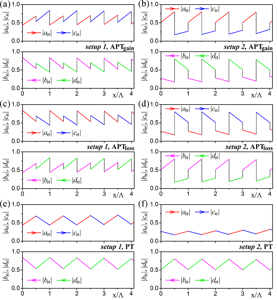
The presented characteristics were made for the two analysed setups and three structures. Curves on the left side of Fig. 4 are drawn for setup 1 and on the right ‒ for setup 2, while Figures 4(a) and 4(b) are for the APT_gain structure; Figures 4(c) and 4(d) are for the APT_loss, and Figures 4(e) and 4(f) are for the PT. For the layers with the refractive index n₁, the wave amplitude |an| (travelling to the right) is coloured red and the wave amplitude |bn| (travelling to the left) is coloured magenta. For the layers with the index n₂, the wave amplitude |cn| (travelling to the right) is marked in blue and the wave amplitude |dn| (travelling to the left) ‒ in green.

Distributions of the field amplitudes shown in Fig. 4 are different for all the investigated setups and structures. These field distributions in all studied structures depend on which layer, with index n₁ or n₂, is excited by incident light. It is worth emphasizing that the distribution of the field

It is worth emphasizing that the distribution of the field amplitudes in the examined structures is strictly related to the values of the refraction indices. In particular, in the APT_gain structure, the distribution of the field amplitudes |an| and |bn| is the same as in the corresponding PT structure, while the distribution of the |cn| and |dn| is reversed in relation to those amplitudes in the PT structure. The opposite situation occurs in the APT_loss structure: the distribution of the field amplitudes |cn| and |dn| is the same as in the corresponding PT structure, while it is reversed for the amplitudes |an| and |bn|. Such a reversal of the field distributions is caused by the negative real part of the refractive index, which can be understood as a reversal of the wave propagation direction.

In general, the wave amplitudes travelling in the structures evolve. A step change is observed at the boundaries, while a monotonic change occurs inside the layers. That step change is larger in both APT structures than in the corresponding PT. This effect is caused by the difference in the refractive indices of both layers forming the ATP structure, wherein one layer, the real part is positive and in the other – negative (see Table 1). However, in the corresponding PT structure, the real parts of the refractive index are the same and the imaginary parts differ in sign.

The waves travelling inside all layers creating the APT_gain structure are amplified in the direction of their propagation, in particular, the amplitudes |an| and |cn| increase with an increase of the current cell number and the amplitudes |bn| and |dn| with a decrease of that number [see Figs. 4(a) and 4(b)]. The opposite situation takes place in the APT_loss structure where the waves are suppressed [see Figs. 4(c) and 4(d)]. Whereas in the corresponding PT structure [see Figs. 4(e) and 4(f)], the travelling waves are alternately amplified (in n₁ layer) and attenuated (in n₂ layer) as they pass through subsequent layers.

Differences in refractive indices characterizing the studied APT_gain, APT_loss, and corresponding PT structures, presented in Table 1, are reflected in different field amplitude distributions. Despite these differences, the reflectance and transmittance of all structures are the same (see Fig. 3). This means that the transfer matrix of the entire structure remains unchanged in relation to the pairs of refractive indices n₁ and n₂.

The presented analysis enables the selection of structural parameters that result in very high transmittance and reflectance values with a small number of primitive cells (as a less complicated case of potential production). Therefore, only structures with a smaller number N of primitive cells, i.e., N = 21, will be included in further analysis.

Nonlinear Case

The nonlinear analysis, including the gain and loss saturation effects, is conducted for both the investigated setups and for the APT_gain, APT_loss, and corresponding PT structures using formulas (6)–(8) from section 2.2 and the procedure presented in Appendix B. In this analysis, meeting two conditions ensuring sufficient accuracy of the calculations required dividing the structure layers into Q = 10 stripes.

Characteristics illustrating the output intensity, transmittance, and reflectance as a function of the input wave intensity were obtained for the setups and structures mentioned above. The parameters correspond to the largest transmission peak from the first row of transmittance maxima (see Table 2). These parameters are: the number of the primitive cells N = 21 and the ratio of the grating period to the operating wavelength Λ/λ = 1.42048. The saturation intensity values selected for the presented analysis are close to realistic values for InP structures [26].

To compare the characteristics of the output intensity, transmittance and reflectance between the APT and the corresponding PT structures, the first step determines the values of the saturation intensity in the gain and loss layers (I_s1 and I_s2, respectively) of the PT structure. Then, in the case of the APT_gain structure, the saturation intensity I_s1 in the layer with the index n₁ is set to the same value as in the PT structure for the gain layer. The saturation intensity I_s2 in the layer with the index n₂ is set to the same value as in the PT structure for the loss layer. The same procedure is followed for selecting the saturation intensity in the APT_loss structure, where the saturation intensity I_s2 in the layer with index n₂ is set to the same value as in the PT structure for the loss layer. Finally, the saturation intensity I_s1 in the layer with the index n₁ is set to the same value as in the PT structure in the gain layer.

Similar to the linear case, the output intensity, transmit-tance, and reflectance characteristics for the selected saturation intensities are the same for all structures: APT_gain, APT_loss, and corresponding PT, despite their different refractive indices. The change in the saturation intensity values modifies the output intensity, transmit-tance, and reflectance characteristics similarly for APT_gain, APT_loss, and corresponding PT structures. The following part of the paper will only show the mentioned characteristics with the saturation intensities selected according to the previously presented procedure.

‌

Fig. 5 shows the dependence of the output intensity I_out({1,2}) as a function of the input intensity for various saturation intensities I_s1 and I_s2 and both setups. The output intensity level I_out({1,2} = 1 W/cm² is marked with a black line.

As anticipated, the output intensity increases in line with the intensity of the input. Moreover, all presented characteristics overlap for very small and very large values of the incident wave intensities, despite of the various saturation intensities I_s1 and I_s2. For the low incident wave intensity (I_in < 10^-7 W/cm²), the observed behaviour is related to negligibly low saturation of the investigated structures. For high incident wave intensities (I_in > 106 W/cm²), it results from a strong saturation of the examined structures, which causes the vanishing of the imaginary part of the refractive indices. This vanishing of the imaginary part causes the medium to become homogeneous. Then, the wave travelling through it does not encounter changes in the refractive index and is neither amplified nor attenuated.

For medium values of the incident wave intensities, the output intensity I_out({1,2}) changes its values depending on the saturation level I_s1 and I_s2, and setups. If the saturation intensity I_s2 is higher than or equal to the saturation intensity I_s1, the output intensity I_out(2) (for setup 2 – the wave leaves the structure through the layer with the refractive index n₁) is higher than I_out(1) (for setup 1 – the wave leaves the structure through the layer with the refractive index n₂). In the case where the saturation intensity I_s2 is equal to the intensity I_s1, the output intensity I_out({1,2}) increases monotonically with the increase of the input wave intensity I_in. An interesting situation occurs when the saturation intensity I_s2 is higher than the intensity I_s1: the output intensity I_out({1,2}) increases rapidly for the input wave intensity I_in close to ten times I_s2: I_in ~ 10 · I_s2. However, when the saturation intensity I_s2 is lower than the intensity I_s1, two areas of the bistability effect appear on the output characteristics for small (I_in ~ 10^-8 · I_s2) and large input wave intensity I_in values (I_in  10 · I_s1). This is caused by the layer with the refractive index n₂ saturating faster. It is worth noting that this is a loss layer in the APT_loss and the corresponding PT structures, whereas in the APT_gain structure the real part of its refractive index is negative.

When the saturation intensity I_s2 is increased while keeping I_s1 constant, the following effects are observed: in Fig. 5(a), the output intensity I_out({1,2}) decreases as the value of I_s2 increases. This is because the layer with index n₂ (loss layer in the corresponding PT structure) absorbs the incident wave more strongly while simultaneously, the layer with index n₁ saturates faster. In Fig. 5(c), the intensity I_out({1,2}) increases with the increase of I_s2, since the layer with index n₁ saturates slower (the intensity I_s1 has the highest value). However, in Fig. 5(b), the increase of the saturation intensity I_s2 causes different changes in the intensity I_out({1,2}) depending on the relationship between intensities I_s1 and I_s2.

‌

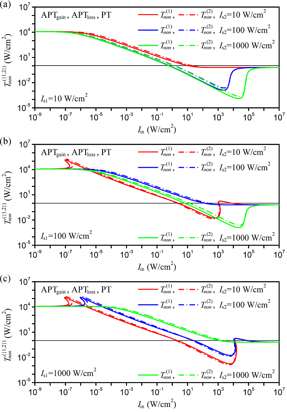
Fig. 6 presents the transmittance T_non({1,2}) as a function of the input intensity for various saturation intensities I_s1 and I_s2 and both setups. Additionally, the transmittance level T_non({1,2}) = 1 is marked with a black line. In general, the transmittance characteristics reflect the output curves of I_out({1,2}) from Fig. 5 because the transmittance is the ratio of the output wave intensity to the incident wave intensity.

It is observed that the transmittance T_non({1,2}) decreases as the intensity of the incident wave I_in increases. Similarly, as the output intensity I_out({1,2}), the transmittance T_non({1,2}) overlaps for very small and very large values of the incident wave intensities despite the various saturation intensities I_s1 and I_s2. The overlapping of T_non({1,2}) characteristics for a very small input intensity I_in corresponds to the situation where the structure is linear and has the same transmittance for both investigated setups. However, in the case of high values of the incident wave intensity I_in, transmittance T_non({1,2}) tends to approach a value of T_non({1,2})  0.64. Once this occurs, the investigated structure becomes saturated and stops behaving like a periodic multi-layer medium. Instead, it starts behaving like a volume medium. As a result, the incident wave is reflected from its two boundaries with the surrounding medium (a medium with coefficient n₀), and the transmittance is equal to T_non({1,2}) = 1 − R_non({1,2}).

For medium values of the incident wave intensities, similarly to the output intensity I_out({1,2}), the transmittance T_non(2) is higher than T_non(1) for the saturation intensity I_s2 higher than or equal to I_s1. When the input intensity I_in is higher than 103 W/cm², and the saturation intensities I_s1 and I_s2 are unequal, the transmittance T_non({1,2}) reaches a minimum and then increases rapidly.

It is important to note that in the case of bistability, when the incident wave I_in is in the range from 10^-7 to 10^-6 W/cm², the transmittance T_non({1,2}) is an order of magnitude larger than the transmittance for a linear structure [see Figs. 6(b) and 6(c)]. On the other hand, for the incident wave I_in in the range from 103 to 104 W/cm², which shows bistability in the output intensity I_out({1,2}), the transmittance T_non({1,2}) reaches the value of two.

‌

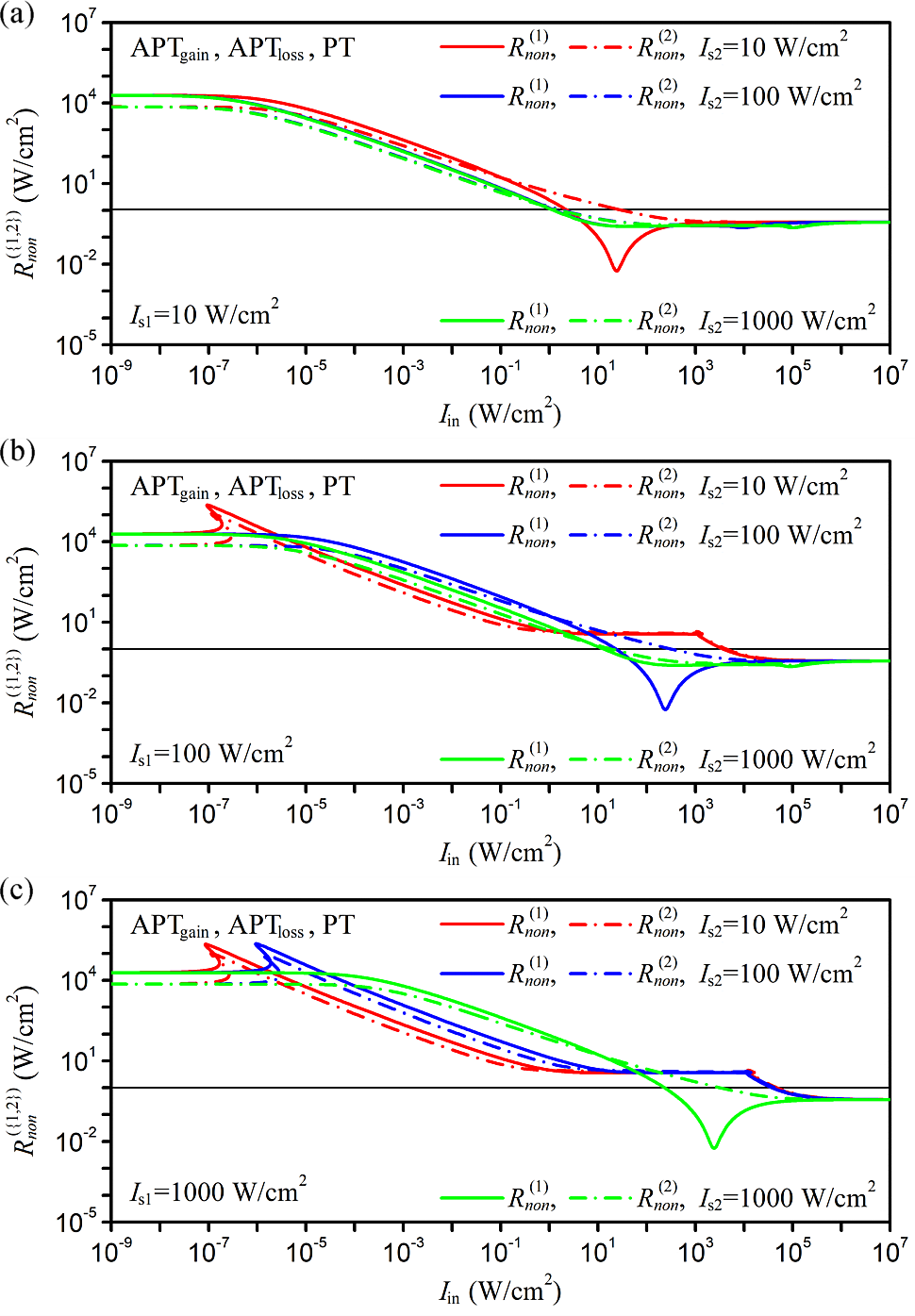
Fig. 7 demonstrates the reflectance R_non({1,2}) as a function of the input intensity for various saturation intensities I_s1 and I_s2 and both setups. Additionally, the reflectance level R_non({1,2}) = 1 is marked with a black line. In general, similar to the transmittances T_non({1,2}), the reflec-tance R_non({1,2}) decreases as the input intensity I_in increases. For very small incident wave intensities, the reflectance R_non({1,2}) behaves as in the linear case and is independent of the saturation intensities I_s1 and I_s2. Moreover, they are different for both setups, with reflectance R_non(1) having a higher value (the incident wave is reflected from the layer with the refractive index n₁) than reflectance R_non(2) indicating nonreciprocity of light propagation. For very large incident wave intensities, the reflectance R_non({1,2}) overlaps and tends to approach a value of R_non({1,2}) ~ 0.36 for the same reasons as transmittance T_non({1,2}).

For medium values of the incident wave intensities, the reflectances for setup 1 are higher than the reflectances for setup 2. The bistability effect occurs for the same saturation intensity pairs I_s1 and I_s2 as in the case of the transmittance. It is worth noting that for equal saturation intensities I_s1 = I_s2, the reflectance R_non(1) reaches its lowest value (global minimum), while the reflectance of R_non(2) is close to unity. This is the unidirectional invisibility effect.

The distribution of the amplitudes |an|, |bn|, |cn|, |dn| for the nonlinear APT_gain, APT_loss, and the corresponding PT structures are shown in Appendix C. Similar to the linear case, these distributions have the same envelope but a different course for each of the examined structures. After considering the gain and loss saturation effect, it is essential to note that the nature of the field distributions in the individual analysed structures remains unchanged. In the APT_gain structure, all amplitudes increase in the direction of the field propagation, in the APT_loss – they decrease and in the corresponding PT structure they alternately increase and decrease.

Conclusions

This work shows the transmittance, reflectance, and output intensity of the multilayer APT symmetric structures as a function of: the input wave intensity for the selected structure period, the primitive cell number, and the saturation intensities. Two setups are investigated: setup 1 – when the wave illuminates the layer with the refractive index n₁ (a gain layer in the corresponding PT structure) and setup 2 – when the wave illuminates the layer with the refractive index n₂ (a loss layer in the PT structure).

The study begins by determining the refractive indices of two types of APT structures: APT_gain with a negative imaginary part of the index and APT_loss with a positive part. These indices are selected with respect to the PT structure. In the case of APT_gain, index n₁ is for the gain layer, similar to the PT structure, whereas index n₂ is selected by the APT condition. In the case of APT_loss, index n₂ is for the loss layer, similar to the PT structure, while index n₁ is selected in accordance with the APT condition.

Next, the linear analysis is performed to determine the APT structures maximal transmittance and reflectance. The results of this analysis are compared with the results of the corresponding analysis of PT structures. Despite the differences between the electromagnetic field distribution of the APT_gain, APT_loss, and PT structures, the reflectance and transmittance characteristics overlap.

The nonlinear analysis uses a modified transfer matrix method which considers the gain and loss saturation effect. This analysis requires a self-consistent method to solve transcendental equations, which allows the matrices describing the transfer of waves through the boundaries of the layers of a primitive cell to be derived. It is worth noting that the refractive indices of all layers depend on the gain and loss saturation effect and influence the wave transmission through the entire structure.

The study examines different gain and loss saturation intensity parameters levels for multilayer APT and corresponding PT structures. The compared structures have the same saturation intensities, I_s1 and I_s2, in their corresponding layers, n₁ and n₂, respectively. Similar to the linear structures, the transmittance, reflectance, and output intensity characteristics are the same for all corresponding structures. Moreover, the obtained characteristics of the output intensities demonstrate a bistable behaviour and are different for both investigated setups. Additionally, the reflectance curves reveal the nonreciprocity of light propagation for small values of the incident wave intensities and the unidirectional invisibility effect for large values of the incident wave intensities. It is worth emphasizing that although APT structures, unlike PT structures, consist of two loss layers or two gain layers, the results obtained for the APT structures are the same as those obtained for classic PT structures. This opens up more possibilities for designing and applying APT structures instead of PT structures. The presented model can be a valuable tool for modelling APT structures and can be applied to various materials.

Authors’ statement

The authors confirm contribution to the paper as follows: research concept and design, A.M.-W. and P.W.; collection and/or assembly of data, A.M.-W. and P.W.; data analysis and interpretation, A.M.-W., P.W., and P.S.; writing the article, A.M.-W., P.W., and P.S.; critical revision of the article, P.S.; final approval of article, A.M.-W., P.W., and P.S.

Acknowledgements

The authors wish to thank Ms. Urszula Wyszyńska for checking the linguistic correctness of the manuscript.

References

1. ‌Ge, L. & Türeci, H. E. Antisymmetric PT-photonic structures with balanced positive- and negative-index materials. Phys. Rev. A. 88, 053810 (2013). https://doi.org/10.1103/PhysRevA.88.053810

2. ‌Bender, C. M. & Boettcher, S. Real spectra in non-Hermitian Hamiltonians having PT symmetry. Phys. Rev. Lett. 80, 5243–5246 (1998). https://doi.org/10.1103/PhysRevLett.80.5243

3. ‌El-Ganainy, R., Makris, K. G., Christodoulides, D. N. & Musslimani,Z. H. Theory of coupled optical PT-symmetric structures. Opt. Lett.3, 2632–2634 (2007). https://doi.org/10.1364/OL.32.002632

4. Cao, H. et al. Unidirectional invisibility induced by complex anti-parity–time symmetric periodic lattices. Appl. Sci. 9, 3808 (2019). ‌https://doi.org/10.3390/app9183808

5. Fang, M., Wang, Y., Zhang, P., Xu, H., & Zhao, D. Multiple exceptional points in APT-symmetric cantor multilayers. Crystals 13, 197 (2023). ‌https://doi.org/10.3390/cryst13020197

6. ‌Shalaev, V. M. Optical negative-index metamaterials. Nat. Photonics 1, 41–48 (2007).

7. Wong, Z. J. Parity-Time Symmetric Laser and Absorber. in Progress in Electromagnetics Research Symposium (PIERS) 1650–1654 (IEEE, 2018). ‌https://doi.org/10.23919/PIERS.2018.8597972

8. Brac de la Perrière, V., Gaimard, Q., Benisty, H., Ramdane, A. & Lupu, A. Electrically injected parity-time symmetric distributed feedback laser diodes (DFB) for telecom applications. Nanophotonics 10, 1309–1317 (2021). ‌https://doi.org/10.1515/nanoph-2020-0587

9. ‌Rüter, C. E. et al. Observation of parity-time symmetry in optics. Nat. Phys. 6, 192–195 (2010). https://doi.org/10.1038/nphys1515

10. Yang, F., Liu, Y.-C. & You, L. Anti-PT symmetry in dissipatively coupled optical systems. Phys. Rev. A 96, 053845 (2017). ‌https://doi.org/10.1103/PhysRevA.96.053845

11. Li, W. et al. Real frequency splitting indirectly coupled anti-parity-time symmetric nanoparticle sensor. J. Appl. Phys. 128, 134503 (2020). ‌https://doi.org/10.1063/5.0020944

12. ‌Passaro, V. M. N. et al. Parity-Time and Anti-Parity-Time- Symmetry Integrated Optical Gyroscopes: A Perspective for High Performance Devices. in 22nd International Conference on Transparent Optical Networks (ICTON) 1–4 (IEEE, 2020). https://doi.org/10.1109/ICTON51198.2020.9203305

13. De Carlo, M. (INVITED) Exceptional points of parity-time- and anti-parity-time-symmetric devices for refractive index and absorption-based sensing. Results Opt. 2, 100052 (2021). ‌https://doi.org/10.1016/j.rio.2020.100052

14. ‌Xu, X.-W., Liao, J.-Q., Jing, H. & Kuang, L.-M. Anti-parity-time symmetry hidden in a damping linear resonator. Sci. China: Phys. Mech. Astron. 66, 100312 (2023).https://doi.org/10.1007/s11433-023-2187-7

15. Fan, H., Chen, J., Zhao, Z., Wen, J. & Huang, Y.-P. Antiparity-time symmetry in passive nanophotonics. ACS Photonics 7, 3035–3041 (2020) ‌https://doi.org/10.1021/acsphotonics.0c01053

16. Zhang, F., Feng, Y., Chen, X., Ge, L. & Wan, W. Synthetic anti-PT symmetry in a single microcavity. Phys. Rev. Lett. 124, 053901 (2020).‌https://doi.org/10.1103/PhysRevLett.124.053901

17. ‌Wei, Y. et al. Anti-parity-time symmetry enabled on-chip chiral polarizer. Photonics Res. 10, 76–83 (2022). https://doi.org/10.1364/PRJ.444075

18. Phang, S. Theory and numerical modelling of parity-time symmetric structures for photonics. (University of Nottingham, 2016). ‌http://eprints.nottingham.ac.uk/32596/

19. Mossakowska-Wyszyńska, A., Witoński, P. & Szczepański, P. Nonlinear operation of an FP laser with PT symmetry active medium. Opt. Express 31, 8518–8534 (2023). ‌https://doi.org/10.1364/OE.479222

20. Witoński, P., Mossakowska-Wyszyńska, A. & Szczepański, P. Gain properties of the single cell of a one-dimensional photonic crystal with PT symmetry. Crystals 13, 258 (2023). ‌https://doi.org/10.3390/cryst13020258

21. Pettit, G. D. & Turner, W. J. Refractive index of InP. J. Appl. Phys. 36, 2081 (1965).‌https://doi.org/10.1063/1.1714410

22. Feng, L., Wong, Z. J., Ma, R.-M., Wang, Y. & Zhang, X. Single-mode laser by parity-time symmetry breaking. Science 346, 972–975 (2014). ‌https://doi.org/10.1126/science.1258479

23. Witoński, P., Mossakowska-Wyszyńska, A. & Szczepański, P. Effect of nonlinear loss and gain in multilayer PT-symmetric Bragg grating. IEEE J. Quantum Electron. 53, 1–11 (2017). https://doi.org/10.1109/JQE.2017.2761380

24. Shramkova, O. V. & Tsironis, G. P. Resonant combinatorial frequency generation induced by a PT-symmetric periodic layered stack. IEEE J. Sel. Top. Quantum Electron. 22, 5000307 (2016). ‌https://doi.org/10.1109/JSTQE.2015.2505139

25. Veselago, V., Braginsky, L., Shklover, V. & Hafner, C. Negative refractive index materials. J. Comput. Theor. Nanosci. 3, 189–218 (2006). ‌https://doi.org/10.1166/jctn.2006.3000

26. Optical Switching in Low-Dimensional Systems. (eds. Haug, H. & Banyai, L.) (Springer USA, 1989). ‌https://doi.org/10.1007/978-1-4684-7278-3

Appendix A

The junction matrices J and the propagation matrices P for linear APT (or PT) structures have the following forms:

matrices J01 (lin) and J10 (lin) describe the behaviour of electromagnetic waves at the boundary between the surrounding medium with coefficient n₀ and the layer with index n₁ for the waves entering and leaving the analysed structure, respectively:

\( \begin{aligned} & J_{01}^{(\text {lin })}=\left[\begin{array}{ll} \frac{n_0+n_1}{2 n_0} & \frac{n_0-n_1}{2 n_0} \\ \frac{n_0-n_1}{2 n_0} & \frac{n_0+n_1}{2 n_0} \end{array}\right], \\ & J_{10}^{(\text {lin })}=\left[\begin{array}{ll} \frac{n_1+n_0}{2 n_1} & \frac{n_1-n_0}{2 n_1} \\ \frac{n_1-n_0}{2 n_1} & \frac{n_1+n_0}{2 n_1} \end{array}\right] ; \end{aligned} \) (A1)

matrices J02 (lin) and J20 (lin) represent the transfer of electromagnetic waves through the boundary between the surrounding medium with coefficient n₀ and the layer with index n₂, for the waves entering and leaving the analysed structure, respectively:

\( \begin{aligned} & J_{02}^{(\text {lin })}=\left[\begin{array}{cc} \frac{n_0+n_2}{2 n_0} & \frac{n_0-n_2}{2 n_0} \\ \frac{n_0-n_2}{2 n_0} & \frac{n_0+n_2}{2 n_0} \end{array}\right], \\ & J_{20}^{(\text {lin })}=\left[\begin{array}{cc} \frac{n_2+n_0}{2 n_2} & \frac{n_2-n_0}{2 n_2} \\ \frac{n_2-n_0}{2 n_2} & \frac{n_2+n_0}{2 n_2} \end{array}\right] ; \end{aligned} \) (A2)

matrices J12 (lin) and J21 (lin) determine the transfer of electromagnetic waves through the boundaries between the layers of the primitive cell and the cell layers adjacent to it, respectively:

\( \begin{aligned} & J_{12}^{(\text {lin })}=\left[\begin{array}{ll} \frac{n_1+n_2}{2 n_1} & \frac{n_1-n_2}{2 n_1} \\ \frac{n_1-n_2}{2 n_1} & \frac{n_1+n_2}{2 n_1} \end{array}\right], \\ & J_{21}^{(\text {lin })}=\left[\begin{array}{ll} \frac{n_2+n_1}{2 n_2} & \frac{n_2-n_1}{2 n_2} \\ \frac{n_2-n_1}{2 n_2} & \frac{n_2+n_1}{2 n_2} \end{array}\right] ; \end{aligned} \) (A3)

matrices P1 (lin) and P2 (lin) describe the propagation of the electromagnetic waves inside the two layers of the primitive cell and are consistent with the relationship:

\( \begin{aligned} & P_1^{(l i n)}=\left[\begin{array}{cc} \mathrm{e}^{-i k_0 n_1 w_a} & 0 \\ 0 & \mathrm{e}^{i k_0 n_1 w_a} \end{array}\right], \\ & P_2^{(l i n)}=\left[\begin{array}{cc} \mathrm{e}^{-i k_0 n_2 w_b} & 0 \\ 0 & \mathrm{e}^{i k_0 n_2 w_b} \end{array}\right] . \end{aligned} \) (A4)

Appendix B

For nonlinear APT (or PT) structures, the matrices P1 (i,non) and P2 (i,non) (describing the propagation of the electromagnetic wave inside the layers of the primitive cell) are different in each i-th stripe of all the layers of the cell and have the following forms:

\( \begin{aligned} & P_1^{(i, n o n)}=\left[\begin{array}{cc} \mathrm{e}^{-i k_0 n_1^{(i)} w_a / Q} & 0 \\ 0 & \mathrm{e}^{i k_0 n_1^{(i)} w_a / Q} \end{array}\right], \\ & P_2^{(i, n o n)}=\left[\begin{array}{cc} \mathrm{e}^{-i k_0 n_2^{(i)} w_b / Q} & 0 \\ 0 & \mathrm{e}^{i k_0 n_2^{(i)} w_b / Q} \end{array}\right], \end{aligned} \) (B1)

where the refractive indices n₁ (i) and n₂ (i) are different for the analysed structures APT_gain, APT_loss, and corresponding PT as follows:

\( \begin{aligned} & n_1^{(i)}\left(a_n^{(i)}, b_n^{(i)}\right)=n_{R e}-i n_{1 I m}^{(i)}\left(a_n^{(i)}, b_n^{(i)}\right), \\ & n_2^{(i)}\left(c_n^{(i)}, d_n^{(i)}\right)=n_{R e}+i n_{2 I m}^{(i)}\left(c_n^{(i)}, d_n^{(i)}\right), \end{aligned} \) (B2)

\( \mathrm{APT}_{\mathrm{gain}}: \begin{gathered} n_1^{(i)}\left(a_n^{(i)}, b_n^{(i)}\right)=n_{R e}-i n_{1 I m}^{(i)}\left(a_n^{(i)}, b_n^{(i)}\right), \\ \\ n_2^{(i)}\left(c_n^{(i)}, d_n^{(i)}\right)=-n_{R e}-i n_{2 I m}^{(i)}\left(c_n^{(i)}, d_n^{(i)}\right), \end{gathered} \) (B3)

\( \begin{array}{ll} & n_1^{(i)}\left(a_n^{(i)}, b_n^{(i)}\right)=-n_{R e}+i n_{1 I m}^{(i)}\left(a_n^{(i)}, b_n^{(i)}\right), \\ & n_2^{(i)}\left(c_n^{(i)}, d_n^{(i)}\right)=n_{R e}+i n_{2 I m}^{(i)}\left(c_n^{(i)}, d_n^{(i)}\right) . \end{array} \) (B4)

The matrices P1 (i,non) and P2 (i,non) in each i-th stripe are related to the complex field amplitudes in the neighbouring stripes:

\( \begin{aligned} & {\left[\begin{array}{l} a_n^{(i-1)} \\ b_n^{(i-1)} \end{array}\right]=P_1^{(i, n o n)}\left[\begin{array}{l} a_n^{(i)} \\ b_n^{(i)} \end{array}\right],} \\ & {\left[\begin{array}{l} c_n^{(i-1)} \\ d_n^{(i-1)} \end{array}\right]=P_2^{(i, n o n)}\left[\begin{array}{c} c_n^{(i)} \\ d_n^{(i)} \end{array}\right] .} \end{aligned} \) (B5)

Therefore, the matrices P1 (non) and P2 (non) are products of the elementary matrices of all the stripes:

\( \begin{aligned} & {\left[\begin{array}{l} a_n^{(0)} \\ b_n^{(0)} \end{array}\right]=\prod_{i=1}^Q P_1^{(i, n o n)}\left[\begin{array}{l} a_n^{(Q)} \\ b_n^{(Q)} \end{array}\right]=P_1^{(\text {non })}\left[\begin{array}{l} a_n^{(Q)} \\ b_n^{(Q)} \end{array}\right],} \\ & {\left[\begin{array}{l} c_n^{(0)} \\ d_n^{(0)} \end{array}\right]=\prod_{i=1}^Q P_2^{(i, n o n)}\left[\begin{array}{l} c_n^{(Q)} \\ d_n^{(Q)} \end{array}\right]=P_2^{(\text {non })}\left[\begin{array}{l} c_n^{(Q)} \\ d_n^{(Q)} \end{array}\right] .} \end{aligned} \) (B6)

The redefinition of matrices J is caused by the change in the longitudinal field distribution due to the gain and loss saturation effect, combining the fields at the boundaries of the cell layers, as shown below [equations (B7(a))–(B9(b))].

When the wave propagates between layers inside a primitive cell, the subscripts in (B9) are defined as m = n. Conversely, when the wave transfers between layers of adjacent cells, the subscripts in (B9) are represented as m = n − 1.

It is important to note that (B8) and (B9) are transcendental, meaning that the field amplitudes on the left side of these equations are simultaneously incorporated within the J matrices on the right side. An approximate solution can only be obtained numerically through the socalled self-consistent method. These equations are solved iteratively, reintegrating the results into the J matrices until the field amplitudes stabilize.

\( \left[\begin{array}{l} c_0 \\ d_0 \end{array}\right]=J_{01}^{(\text {non })}\left[\begin{array}{l} a_1^{(0)} \\ b_1^{(0)} \end{array}\right]=\left[\begin{array}{ll} \frac{n_0+n_1^{(0)}\left(a_1^{(0)}, b_1^{(0)}\right)}{2 n_0} & \frac{n_0-n_1^{(0)}\left(a_1^{(0)}, b_1^{(0)}\right)}{2 n_0} \\ \frac{n_0-n_1^{(0)}\left(a_1^{(0)}, b_1^{(0)}\right)}{2 n_0} & \frac{n_0+n_1^{(0)}\left(a_1^{(0)}, b_1^{(0)}\right)}{2 n_0} \end{array}\right]\left[\begin{array}{l} a_1^{(0)} \\ b_1^{(0)} \end{array}\right], \) (B7a)

\( \left[\begin{array}{l} a_0 \\ b_0 \end{array}\right]=J_{02}^{(\text {non })}\left[\begin{array}{l} c_1^{(0)} \\ d_1^{(0)} \end{array}\right]=\left[\begin{array}{ll} \frac{n_0+n_2^{(0)}\left(c_1^{(0)}, d_1^{(0)}\right)}{2 n_0} & \frac{n_0-n_2^{(0)}\left(c_1^{(0)}, d_1^{(0)}\right)}{2 n_0} \\ \frac{n_0-n_2^{(0)}\left(c_1^{(0)}, d_1^{(0)}\right)}{2 n_0} & \frac{n_0+n_2^{(0)}\left(c_1^{(0)}, d_1^{(0)}\right)}{2 n_0} \end{array}\right]\left[\begin{array}{l} c_1^{(0)} \\ d_1^{(0)} \end{array}\right], \) (B7b)

\( \left[\begin{array}{c} c_N^{(\varrho)} \\ d_N^{(\varrho)} \end{array}\right]=J_{20}^{(n o n)}\left[\begin{array}{c} a_{N+1} \\ 0 \end{array}\right]=\left[\begin{array}{ll} \frac{n_2^{(\varrho)}\left(c_N^{(\varrho)}, d_N^{(\varrho)}\right)+n_0}{2 n_2^{(\varrho)}\left(c_N^{(\varrho)}, d_N^{(\varrho)}\right)} & \frac{n_2^{(\varrho)}\left(c_N^{(\varrho)}, d_N^{(\varrho)}\right)-n_0}{2 n_2^{(\varrho)}\left(c_N^{(\varrho)}, d_N^{(\varrho)}\right)} \\ \frac{n_2^{(\varrho)}\left(c_N^{(\varrho)}, d_N^{(\varrho)}\right)-n_0}{2 n_2^{(\varrho)}\left(c_N^{(\varrho)}, d_N^{(\varrho)}\right)} & \frac{n_2^{(\varrho)}\left(c_N^{(\varrho)}, d_N^{(\varrho)}\right)+n_0}{2 n_2^{(\varrho)}\left(c_N^{(\varrho)}, d_N^{(\varrho)}\right)} \end{array}\right]\left[\begin{array}{c} a_{N+1} \\ 0 \end{array}\right], \) (B8a)

\( \left[\begin{array}{l} a_N^{(\varrho)} \\ b_N^{(\varrho)} \end{array}\right]=J_{10}^{(n o n)}\left[\begin{array}{c} c_{N+1} \\ 0 \end{array}\right]=\left[\begin{array}{ll} \frac{n_1^{(Q)}\left(a_N^{(\varrho)}, b_N^{(Q)}\right)+n_0}{2 n_1^{(Q)}\left(a_N^{(\varrho)}, b_N^{(Q)}\right)} & \frac{n_1^{(Q)}\left(a_N^{(\varrho)}, b_N^{(Q)}\right)-n_0}{2 n_1^{(Q)}\left(a_N^{(\varrho)}, b_N^{(Q)}\right)} \\ \frac{n_1^{(Q)}\left(a_N^{(\varrho)}, b_N^{(Q)}\right)-n_0}{2 n_1^{(Q)}\left(a_N^{(Q)}, b_N^{(Q)}\right)} & \frac{n_1^{(Q)}\left(a_N^{(\varrho)}, b_N^{(Q)}\right)+n_0}{2 n_1^{(Q)}\left(a_N^{(Q)}, b_N^{(Q)}\right)} \end{array}\right]\left[\begin{array}{c} c_{N+1} \\ 0 \end{array}\right], \) (B8b)

\( \left[\begin{array}{l} a_m^{(Q)} \\ b_m^{(Q)} \end{array}\right]=J_{12}^{(n o n)}\left[\begin{array}{l} c_n^{(0)} \\ d_n^{(0)} \end{array}\right]=\left[\begin{array}{cc} \frac{n_1^{(Q)}\left(a_m^{(Q)}, b_m^{(Q)}\right)+n_2^{(0)}\left(c_n^{(0)}, d_n^{(0)}\right)}{2 n_1^{(Q)}\left(a_m^{(Q)}, b_m^{(Q)}\right)} & \frac{n_1^{(Q)}\left(a_m^{(Q)}, b_m^{(Q)}\right)-n_2^{(0)}\left(c_n^{(0)}, d_n^{(0)}\right)}{2 n_1^{(Q)}\left(a_m^{(Q)}, b_m^{(Q)}\right)} \\ \frac{n_1^{(Q)}\left(a_m^{(Q)}, b_m^{(Q)}\right)-n_2^{(0)}\left(c_n^{(0)}, d_n^{(0)}\right)}{2 n_1^{(Q)}\left(a_m^{(Q)}, b_m^{(Q)}\right)} & \frac{n_1^{(Q)}\left(a_m^{(Q)}, b_m^{(Q)}\right)+n_2^{(0)}\left(c_n^{(0)}, d_n^{(0)}\right)}{2 n_1^{(Q)}\left(a_m^{(Q)}, b_m^{(Q)}\right)} \end{array}\right]\left[\begin{array}{l} c_n^{(0)} \\ d_n^{(0)} \end{array}\right] \) (B9a)

\( \left[\begin{array}{l} c_m^{(Q)} \\ d_m^{(Q)} \end{array}\right]=J_{21}^{(n o n)}\left[\begin{array}{l} a_n^{(0)} \\ b_n^{(0)} \end{array}\right]=\left[\begin{array}{ll} \frac{n_2^{(Q)}\left(c_m^{(Q)}, d_m^{(Q)}\right)+n_1^{(0)}\left(a_n^{(0)}, b_n^{(0)}\right)}{2 n_2^{(\varrho)}\left(c_m^{(Q)}, d_m^{(Q)}\right)} & \frac{n_2^{(Q)}\left(c_m^{(Q)}, d_m^{(Q)}\right)-n_1^{(0)}\left(a_n^{(0)}, b_n^{(0)}\right)}{2 n_2^{(Q)}\left(c_m^{(Q)}, d_m^{(Q)}\right)} \\ \frac{n_2^{(Q)}\left(c_m^{(Q)}, d_m^{(Q)}\right)-n_1^{(0)}\left(a_n^{(0)}, b_n^{(0)}\right)}{2 n_2^{(Q)}\left(c_m^{(Q)}, d_m^{(Q)}\right)} & \frac{n_2^{(Q)}\left(c_m^{(Q)}, d_m^{(Q)}\right)+n_1^{(0)}\left(a_n^{(0)}, b_n^{(0)}\right)}{2 n_2^{(Q)}\left(c_m^{(Q)}, d_m^{(Q)}\right)} \end{array}\right]\left[\begin{array}{l} a_n^{(0)} \\ b_n^{(0)} \end{array}\right] . \) (B9b)

To determine the intensities of the output waves I_out(1) and I_out(2) for the APT_gain, APT_loss, and corresponding PT structures as functions of the incident plane waves intensities I_in (1) and I_in (2) (see Fig. 1), the following procedure is used. The relevant values for setup 1 are explicitly provided, while those for setup 2 are indicated in parentheses.

Step 1. Select the parameters of the investigated structure, including the number of primitive cells N and the period of the structure normalized to the length of the analysed wave . The saturation intensity values I_s1 and I_s2 and the number Q of stripes are assumed for both layers. Assuming that the wave is incident from one side of the structure, the complex amplitude of the output wave is defined as I_out(1) = |aN+1|² (I_out(2) = |cN+1|²).

Step 2. Use transcendental (B8) to calculate the amplitudes cN(Q) and dN(Q) (aN(Q) and bN(Q)) in the Q-th stripe of the last layer n₂ (n₁) of N-th cell at the boundary with the medium of refractive index n₀.

Step 3. Employ the amplitudes obtained in Step 2 to calculate cN(0) and dN(0) (aN(0) and bN(0)) using (B6). This step iteratively computes the distribution of wave amplitudes in the investigated layer with coefficient n₂ (n₁) in the second layer of the last cell.

Step 4. Using transcendental (B9) and the amplitudes from Step 3, calculate the amplitudes an(Q) and bn(Q) (cn(Q) and dn(Q)) in the Q-th stripe of the layer n₁ (n₂) adjacent to the second layer of n-th cell, where n = N in the last cell.

Step 5. With the amplitudes obtained in Step 4, calculate an(0) and bn(0) (cn(0) and dn(0)) using (B6). This iterative calculation determines the distribution of wave amplitudes in the investigated layer with coefficient n₁ (n₂).

Step 6. Using transcendental (B9) and the amplitudes from Step 5, calculate the amplitudes cn(Q) and dn(Q) (an(Q) and bn(Q)) in the Q-th stripe of the layer n₂ (n₁).

Step 7. With the amplitudes obtained in Step 6, calculate the amplitudes cn(0) and dn(0) (an(0) and bn(0)) using (B6). This process iteratively determines the distribution of wave amplitudes in the investigated layer with coefficient n₂ (n₁).

Step 8. Using transcendental (B9) and the amplitudes from Step 7, calculate the amplitudes an(Q) and bn(Q) (cn(Q) and dn(Q)) in the Q-th stripe of the layer n₁ (n₂) adjacent to the second layer of n-th cell, where n = 1 in the first cell.

Step 9. Repeat the calculations from Steps 5 to 8 until the wave amplitudes are determined in all primitive cells of the investigated structure.

Step 10. Using the amplitudes obtained in Step 9, calculate a1(0) and b1(0) (c1(0) and d1(0)) using (B6). This iterative process determines the distribution of wave amplitudes in the investigated layer with coefficient n₁ (n₂) in the first layer of the first cell.

Step 11. Using transcendental (B7) and the amplitudes from Step 10, calculate the amplitudes c0 and d0 (a0 and b0) in the medium with refractive index n₀. The resulting field amplitudes allow to determine the incident wave intensity I_in(1) (I_in(2)) and the reflected wave intensity Ir(1) (Ir(2)).

Appendix C

The field amplitudes of counter running waves |an|, |bn|, |cn|, |dn|, within all primitive cells forming the nonlinear structures: APT_gain, APT_loss, and corresponding PT are shown in Figs. 8, 9, and 10, respectively.

These charts are derived assuming that output intensity equals I_out({1,2}) = 1 W/cm², corresponding to one point on the output characteristics in Fig. 5. Characteristics shown in Figs. 8, 9, and 10 are plotted for setup 1 in the left columns and setup 2 in the right columns, with two pairs of saturation intensities: the top rows representing I_s1 = 10 W/cm² and I_s2 = 1000 W/cm², and the bottom rows representing I_s1 = 1000 W/cm² and I_s2 = 10 W/cm². These figures are presented for the structural parameters corresponding to the largest transmission peak from the first row of maxima in the linear case, i.e., N = 21 and  = 1.42048 (see Table 2).

‌

Similar to the linear case, the envelopes of the curves for each setup and pair of saturation intensities are consistent across all types of structures. For instance, the field amplitude envelopes shown in Fig. 8(a) can be compared with those in Fig. 9(a) and Fig. 10(a) and similarly for the other subfigures. However, the field distributions vary for each examined structure and are highly dependent on the level of saturation intensities. It is important to note that after accounting for the gain and loss saturation effect, the nature of the field distributions in the individual structures remains unchanged. In the APT_gain structure, all amplitudes increase along the direction of the field propagation; in the APT_loss structure, they decrease; and in the corresponding PT structure, they alternate between increasing and decreasing.

‌

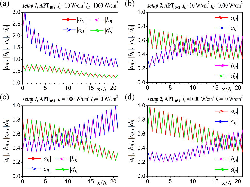
Moreover, accounting for the gain and loss saturation effect changes the field amplitude values. The biggest differences are observed between setup 1 and setup 2 for the first pair of saturation intensities (I_s1 = 10 W/cm² and I_s2 = 1000 W/cm²). To achieve the output intensity I_out({1,2}) = 1 W/cm², waves I_in with a different intensity must be applied to the structures. In the examined case, the wave entering setup 1 is an order of magnitude larger than the wave I_in for setup 2 [see Fig. 5(a)]. This effect is due to the differing electromagnetic wave distributions within the investigated structures, as seen by comparing subfigure (a) with subfigure (b) in Figs. 8, 9, and 10 for the APT_gain, APT_loss, and PT structures, respectively.

‌

A different situation is observed for the second pair of saturation intensities, I_s1 = 1000 W/cm² and I_s2 = 10 W/cm². Comparing subfigure (c) with subfigure (d) in Figs. 8, 9, and 10 for the APT_gain, APT_loss, and corresponding PT structures, respectively, reveals that for these saturation intensities, achieving an output wave intensity I_out({1,2}) = 1 W/cm² requires excitation with a wave of a similar value for both setups [see Fig. 5(c)]. This outcome corresponds to the longitudinal field distribution within all the examined structures.